Setting up a database
Introduction
In this assignment, you'll perform few basic tasks needed to create a database. You'll design the tables create it, add indexes to them and of course connect everything with appropriate relations. You also learn how to use LOAD DB2 Utility. The database we'll create will be used for storing RMF performance data. It will consist of three tables: - LPARS – Each record stores some basic information about a single LPAR. - PERF_RMF_INT – Each record represents RMF performance data from a single interval. It depends on RMF setting, usually, RMF saves the data each 10, 15 or 30 minutes. - PERF_DAY_AVG – Each record stores daily average values of selected columns from PERF_RMF_INT table. Before starting this Assignment contact your database administrator or RACF support (depending on how the DB2 is protected) in order to get appropriate authorization for DB2 operations.
Tasks
![]() 1. Create a database and a single tablespace in it.
1. Create a database and a single tablespace in it.
![]() 2. Design three tables described in the introduction: LPARS, PERF_RMF_INT and PERF_DAY_AVG.
- Hint 2 contains JCL code for a sample RMF job that extracts fields that will be stored in PERF_RMF_INT table. You can model your tables on it or modify the job and then design the table accordingly. It is recommended you use the same job since solutions of many later Tasks will depend on the data gathered by RMF.
- There are many free tools in which you can create rational database diagrams and then generate SQL for the database creation. You'll save a lot of time this way.
2. Design three tables described in the introduction: LPARS, PERF_RMF_INT and PERF_DAY_AVG.
- Hint 2 contains JCL code for a sample RMF job that extracts fields that will be stored in PERF_RMF_INT table. You can model your tables on it or modify the job and then design the table accordingly. It is recommended you use the same job since solutions of many later Tasks will depend on the data gathered by RMF.
- There are many free tools in which you can create rational database diagrams and then generate SQL for the database creation. You'll save a lot of time this way.
![]() 3. Create tables designed in Task#2 and join them with appropriate relations.
3. Create tables designed in Task#2 and join them with appropriate relations.
![]() 4. Manually insert two records into LPAR table.
4. Manually insert two records into LPAR table.
![]() 5. Run RMF job that creates Overview report from the selected system resources.
- Sample JCL code is in Hint 2.
- Make sure that RMF control statements match columns in your database.
5. Run RMF job that creates Overview report from the selected system resources.
- Sample JCL code is in Hint 2.
- Make sure that RMF control statements match columns in your database.
![]() 6. Reformat RMF report with DFSORT so it can be processed by DB2 LOAD Utility.
6. Reformat RMF report with DFSORT so it can be processed by DB2 LOAD Utility.
![]() 7. Use DB2 LOAD Utility to load RMF data into PERF_RMF_INT table.
7. Use DB2 LOAD Utility to load RMF data into PERF_RMF_INT table.
Hint 1
DB2 documentation is available under the following address: http://www-01.ibm.com/support/docview.wss?uid=swg27039165 For this Task, “DB2 11 for z/OS: SQL Reference” and “DB2 11 for z/OS: Introduction to DB2 for z/OS” are two documents that will be helpful. Be sure to check “Appendix: DB2 catalog tables” in “DB2 11 for z/OS: SQL Reference”. It contains description of build-in DB2 tables which you'll have to get familiar with. When it comes to running SQL queries two tools are usually used: - SPUFI – This is a build-in function of DB2I (DB2 Interactive), the default interface for running SQL queries. - DB2 QMF – Query Management Facility is another popular tool. This assignment does not cover those tools but both of them are easy to figure out.
Hint 2
JCL Code for RMF report:
//SMFSORT EXEC PGM=SORT,REGION=0M //SORTIN DD DISP=SHR,DSN=&SYSUID..SMF.DUMP1 <-- SMF DATA // DD DISP=SHR,DSN=&SYSUID..SMF.DUMP2 //SORTOUT DD DISP=(,PASS),SPACE=(CYL,(200,200),RLSE),DSN=&PLXG //SORTWK01 DD DISP=(NEW,DELETE),UNIT=3390,SPACE=(CYL,(200)) //SORTWK02 DD DISP=(NEW,DELETE),UNIT=3390,SPACE=(CYL,(200)) //SORTWK03 DD DISP=(NEW,DELETE),UNIT=3390,SPACE=(CYL,(200)) //SORTWK04 DD DISP=(NEW,DELETE),UNIT=3390,SPACE=(CYL,(200)) //SORTWK05 DD DISP=(NEW,DELETE),UNIT=3390,SPACE=(CYL,(200)) //SORTWK06 DD DISP=(NEW,DELETE),UNIT=3390,SPACE=(CYL,(200)) //SORTWK07 DD DISP=(NEW,DELETE),UNIT=3390,SPACE=(CYL,(200)) //SORTWK08 DD DISP=(NEW,DELETE),UNIT=3390,SPACE=(CYL,(200)) //SYSPRINT DD SYSOUT=* //SYSOUT DD SYSOUT=* //SYSIN DD * SORT FIELDS=(11,4,CH,A,7,4,CH,A),EQUALS MODS E15=(ERBPPE15,36000,,N),E35=(ERBPPE35,3000,,N) //RMFPP EXEC PGM=ERBRMFPP,REGION=512M //MFPINPUT DD DSN=&PLXG,DISP=(OLD,PASS) //MFPMSGDS DD SYSOUT=* //PPOVWREC DD DISP=(,CATLG),DSN=&SYSUID..RMF.FULL, <-- OUTPUT // SPACE=(CYL,(50,50),RLSE),BLKSIZE=0,UNIT=SYSDA //PPORP001 DD SYSOUT=* //SYSPRINT DD SYSOUT=* //SYSOUT DD SYSOUT=* //SYSIN DD * <-- SUPPLY LPAR NAME DATE(07312017,08062017) OVERVIEW(RECORD,REPORT) NOSUMMARY /* CPU */ OVW(CPUBSY(CPUBSY)) /* PHYSICAL CP BUSY */ OVW(IIPBSY(IIPBSY)) /* PHYSICAL ZIIP BUSY */ OVW(MVSBSY(MVSBSY)) /* MVS CP BUSY */ OVW(IIPMBSY(IIPMBSY)) /* MVS ZIIP BUSY */ OVW(AVGWUCP(AVGWUCP)) /* INREADY QUEUE FOR CP */ OVW(AVGWUIIP(AVGWUIIP)) /* INREADY QUEUE FOR ZIIP */ OVW(NLDEFL(NLDEFL(PZ13))) /* DEF PROCESSORS IN PARTITION */ OVW(NLDEFLCP(NLDEFLCP(PZ13))) /* DEF CP IN PARTITION */ OVW(NLDEFLIP(NLDEFLIP(PZ13))) /* DEF ZIIP IN PARTITION */ OVW(NLACTL(NLACTL(PZ13))) /* ACTUAL PROCESSORS IN PARTITION */ OVW(NLACTLCP(NLACTLCP(PZ13))) /* ACTUAL CP IN PARTITION */ OVW(NLACTLIP(NLACTLIP(PZ13))) /* ACTUAL ZIIP IN PARTITION */ /* MSU */ OVW(WDEFL(WDEFL(PZ13))) /* DEF WEIGHTS FOR CP */ OVW(WDEFLIIP(WDEFLIIP(PZ13))) /* DEF WEIGHTS FOR ZIIP */ OVW(WACTL(WACTL(PZ13))) /* ACTUAL WEIGHTS FOR CP */ OVW(LDEFMSU(LDEFMSU(PZ13))) /* DEFINED MSU */ OVW(LACTMSU(LACTMSU(PZ13))) /* USED MSU */ OVW(WCAPPER(WCAPPER(PZ13))) /* WLM CAPPING */ OVW(INICAP(INICAP(PZ13))) /* INITIAL CAPPING FOR THE CP */ OVW(LIMCPU(LIMCPU(PZ13))) /* PHYSICAL HW CAPACITY LIMIT */ /* STORAGE */ OVW(STOTOT(STOTOT(POLICY))) /* USED CENTRAL STORAGE */ OVW(STORAGE(STORAGE)) /* AVAILABLE CENTRAL STORAGE */ OVW(TPAGRT(TPAGRT)) /* PAGE-INS & PAGE-OUTS PER SEC */ OVW(PAGERT(PAGERT)) /* PAGE FAULTS */ OVW(PGMVRT(PGMVRT)) /* PAGE MOVE RATE */ OVW(CSTORAVA(CSTORAVA)) /* AVG NUMBER OF ALL FRAMES */ OVW(AVGSQA(AVGSQA)) /* AVG NUMBER OF SQA FIXED FRAMES */ OVW(AVGCSAF(AVGCSAF)) /* AVG NUMBER OF CSA FIXED FRAMES */ OVW(AVGCSAT(AVGCSAT)) /* AVG NUMBER OF ALL CSA FRAMES */ /* I/O */ OVW(IOPIPB(IOPIPB)) /* I/O PROCESOR BUSY PERCENT */ OVW(IORPII(IORPII)) /* RATE OF PROCESSED I/O INTERRUPTS */ OVW(IOPALB(IOPALB)) /* PERCENT OF I/O RETRIES */
RMF overview reports saves extracted data in form of columns and rows so just like a table in relational database. Thanks to that you can easily map OVW statements into table definition. The easiest and fastest way to design table diagram is to use one of the freeware database designers. Each of them provides graphical interface through which you can create your tables and relationships between them. Make sure that the tool you're using supports DB2 SQL version.
Hint 3
Each Database Design Tool can generate SQL code from the diagram you've created. Basically there are four things to do: - Tables creation. - Indexes creation. - Primary keys definition. - Foreign keys definition.
Hint 6
You'll have to omit some records and also at least one column. You'll also have to reformat Date format in RMF report so it's in format readable by DB2 LOAD Utility. See OMIT & OUTREC control statements of DFSORT Utility. It's documented in “z/OS DFSORT Application Programming Guide”.
Hint 7
In “DB2 11 for z/OS: Introduction to DB2 for z/OS” there is "Chapter 10. DB2 basics tutorial" where LOAD Utility is briefly described. For more details be sure to check "Db2 11 for z/OS: Utility Guide and Reference".
Solution 1
The first thing to do is to ensure you have an appropriate authorization to the DB2 subsystem. DB2 can be protected in two ways, via DB2 Authorization Table or RACF profiles. Depending on that it may be controlled either by DBDC or RACF team, you may need to contact them to be able to finish this Assignment. Creation of database is very simple. This is only it's definition so we don't have to worry about details. CREATE DATABASE JANSDB; You can display all databases defined in particular DB2 subsystem with SQL command: SELECT * FROM SYSIBM.SYSDATABASE; Table space is a physical file (VSAM LDS) in which your tables and the data in them will be stored. You can create it as follows:
CREATE TABLESPACE JANSTS1 IN JANSDB USING STOGROUP SYSDEFLT PRIQTY 3000 SECQTY 3000 ERASE YES CCSID ASCII LOCKSIZE ROW;
STOGROUP has nothing to do with SMS Storage group. This is simply a list of volumes which DB2 will use for allocating your table space. You can display available storage groups with: SELECT * FROM SYSIBM.SYSSTOGROUP; To display what volume will be chosen by selecting SYSDEFLT group you can issue: SELECT * FROM SYSIBM.SYSVOLUMES WHERE SGNAME='SYSDEFLT'; If you have access do “DB2 Admin” you can also view Catalog Tables via option 1 (DB2 system catalog). PRIQTY and SECQTY define how large your table space can be. They are specified in Pages, a Page can have from 4kB up to 32kB, 4kB is the default.
Solution 2
Three tables have to be created: - LPAR - PERF_RMF_INT - PERF_DAY_AVG First one is for general information about LPAR and the other two are for storing data extracted by the job included in Hint 2. First let's check what built-in data types are available in DB2: Numeric: - SMALLINT - -32768 to +32767 - INTEGER - -2147483648 to +2147483647 - BIGINT - -9223372036854775808 to +9223372036854775807 - REAL - 32 bit floating point - DOUBLE - (or FLOAT) 64 bit floating point - DECIMAL - (or NUMERIC) decimal floating point - max 31 digits - DECFLOAT - decimal floating point - max 34 digits String: - CHAR(n) - fixed length string (max 255 characters) - VARCHAR(n) - variable length string (max 32704 characters) - CLOB(n) - variable length string (max 2147483647 characters) - GRAPHIC(n) - fixed length double-byte string (max 127 characters) - VARGRAPHIC(n) - variable length double-byte string (max 16352 characters) - DBCLOB(n) - variable length double-byte string (max 1073741823 characters) - BINARY(n) - fixed length binary string (max 127 characters) - VARBINARY(n) - variable length binary string (max 32704 characters) - BLOB(n) - variable length binary string (max 2147483647 characters) Date and time - DATE - Date - TIME - Time - TIMESTAMP WITHOUT TIME ZONE - Date & Time & Fractional (GMT time zone) - TIMESTAMP WITH TIME ZONE - Date & Time & Fractional (Local time zone) OTHER: - ROWID - ID of a record - XML - Formatted XML string (max 2147483647 characters) In “Data Types” chapter of “DB2 11 for z/OS: SQL Reference” there is a table that nicely shows all built-in data types. Here are few remarks regarding types: 1. User created types are also supported, they're called Distinct types. 2. The difference between three types of strings: - Normal character strings - For storing data in ASCII or EBCDIC format. The format can be defined in data base, table space or table definition. - Double-byte character strings - For storing data in UTF-16 format. - Binary character strings - For storing binary data, for example sounds or pictures. 3. Binary vs Decimal representation of numbers: - Floating point numbers are not precise. This is the main reason why Decimal are recommended. - When moving data to system other than mainframe floating point numbers may be coded differently. In such case, conversion is needed. - Mainframes processors have special hardware circuits for processing Decimal numbers while other processors must first convert them to a binary form. This means that if you need to process a lot of data on systems other than mainframe floating point calculations are faster. - Floating-point numbers take less storage than decimal. - DECFLOAT is simply a DECIMAL representation with more precision. It is a relatively new type, added in DB2 9, because of that it's best to stick with DECIMAL for compatibility reasons. Database diagram (made with use of dbdiffo.com online editor):

As you can see PERF_RMF_INT table will store all the information extracted by RMF job. PERF_DAY_AVG stores only selected columns. The idea is simple, PERF_RMF_INT will store all RMF intervals for like a month of two. This way a System Programmer will be able to easily analyze the detailed performance data from the last few weeks/months. RMF itself retains such data only for a few days. PERF_DAY_AVG is a table in which one row represents a single day, this data will be stored for a longer period, for example 5 years. It's standard practice to store some SMF data for many years, for example MIPS & MSU usage, SMF record 89 etc. Such data may be needed for pricing software or long term performance analysis. There are three Foreign Key constraints between those tables: - DAY_AVG_FK_LPAR – 1 to 0-n – one LPAR can have zero or more PERF_DAY_AVG records and each PERF_DAY_AVG record must be connected to a single LPAR record. - RMF_INT_FK_LPAR – 1 to 0-n – one LPAR can have zero or more PERF_RMF_INT records and each PERF_RMF_INT record must be connected to a single LPAR record. - RMF_INT_FK_DAY_AVG - 0,1 to 0-n – one PERF_DAY_AVG record may have zero or more PERF_RMF_INT records and one PERF_RMF_INT record may or may not be connected to a single RMF_DAY_AVG record.
Solution 3
SQL code for LPAR table:
CREATE TABLE LPAR ( LPAR_ID SMALLINT NOT NULL GENERATED BY DEFAULT AS IDENTITY (START WITH 1, INCREMENT BY 1), LPAR_NAME VARCHAR(4) NOT NULL, CPU_MODEL VARCHAR(10) NOT NULL, Z_OS_VERSION VARCHAR(6) NOT NULL, MAINTANANCE_LEVEL DATE NOT NULL, KEEP_RMFINT_FOR_X_DAYS SMALLINT NOT NULL DEFAULT 40, KEEP_DAYAVG_FOR_X_DAYS SMALLINT NOT NULL DEFAULT 2000, COMPANY_NAME VARCHAR(50), COMMENTS VARCHAR(500) ) IN JANSDB.JANSTS1; CREATE UNIQUE INDEX IX1_LPAR ON LPAR (LPAR_ID ASC) USING STOGROUP SYSDEFLT PRIQTY 64 SECQTY 64 ERASE YES BUFFERPOOL BP2 CLOSE YES; ALTER TABLE LPAR ADD CONSTRAINT LPAR_ID PRIMARY KEY (LPAR_ID);
SQL code was generated automatically by “dbdiffo.com” website, there are two modifications: - IN JANSDB.JANSTS1 – remember to add it in CREATE TABLE statement, otherwise DB2 will create the table in new automatically generated database. - CREATE UNIQUE INDEX – creating index is optional and not really needed in this assignment but all production databases use Indexes so it's good habit to always create it, just to get used to it. SQL code for PERF_DAY_AVG table:
CREATE TABLE PERF_DAY_AVG ( PERF_DAY_AVG_ID INTEGER NOT NULL GENERATED BY DEFAULT AS IDENTITY (START WITH 1, INCREMENT BY 1), LPAR_ID SMALLINT NOT NULL, DATE DATE NOT NULL, CPUBSY DECIMAL(6,3) NOT NULL DEFAULT 0, IIPBSY DECIMAL(6,3) NOT NULL DEFAULT 0, MVSBSY DECIMAL(6,3) NOT NULL DEFAULT 0, IIPMBSY DECIMAL(6,3) NOT NULL DEFAULT 0, AVGWUCP DECIMAL(6,3) NOT NULL DEFAULT 0, AVGWUIIP DECIMAL(6,3) NOT NULL DEFAULT 0, WDEFL DECIMAL(6,0) NOT NULL DEFAULT 0, WDEFLIIP DECIMAL(6,0) NOT NULL DEFAULT 0, WACTL DECIMAL(6,0) NOT NULL DEFAULT 0, LDEFMSU DECIMAL(6,0) NOT NULL DEFAULT 0, LACTMSU DECIMAL(6,0) NOT NULL DEFAULT 0, STOTOT DECIMAL(15,0) NOT NULL DEFAULT 0, TPAGRT DECIMAL(15,3) NOT NULL DEFAULT 0, IORPII DECIMAL(15,3) NOT NULL DEFAULT 0, IOPALB DECIMAL(15,3) NOT NULL DEFAULT 0 ) IN JANSDB.JANSTS1; CREATE UNIQUE INDEX IX1_PERF_DAY_AVG ON PERF_DAY_AVG (PERF_DAY_AVG_ID ASC) USING STOGROUP SYSDEFLT PRIQTY 64 SECQTY 64 ERASE YES BUFFERPOOL BP2 CLOSE YES; ALTER TABLE PERF_DAY_AVG ADD CONSTRAINT PERF_DAY_AVG_ID PRIMARY KEY (PERF_DAY_AVG_ID);
SQL code for PERF_RMF_INT table:
CREATE TABLE PERF_RMF_INT ( PERF_RMF_INT_ID INTEGER NOT NULL GENERATED BY DEFAULT AS IDENTITY (START WITH 1, INCREMENT BY 1), LPAR_ID SMALLINT NOT NULL, PERF_DAY_AVG_ID INTEGER, DATE DATE NOT NULL, TIME TIME NOT NULL, CPUBSY DECIMAL(6,3) NOT NULL DEFAULT 0, IIPBSY DECIMAL(6,3) NOT NULL DEFAULT 0, MVSBSY DECIMAL(6,3) NOT NULL DEFAULT 0, IIPMBSY DECIMAL(6,3) NOT NULL DEFAULT 0, AVGWUCP DECIMAL(6,3) NOT NULL DEFAULT 0, AVGWUIIP DECIMAL(6,3) NOT NULL DEFAULT 0, NLDEFL DECIMAL(3,0) NOT NULL DEFAULT 0, NLDEFLCP DECIMAL(3,0) NOT NULL DEFAULT 0, NLDEFLIP DECIMAL(3,0) NOT NULL DEFAULT 0, NLACTL DECIMAL(3,0) NOT NULL DEFAULT 0, NLACTLCP DECIMAL(3,0) NOT NULL DEFAULT 0, NLACTLIP DECIMAL(3,0) NOT NULL DEFAULT 0, WDEFL DECIMAL(6,0) NOT NULL DEFAULT 0, WDEFLIIP DECIMAL(6,0) NOT NULL DEFAULT 0, WACTL DECIMAL(6,0) NOT NULL DEFAULT 0, LDEFMSU DECIMAL(6,0) NOT NULL DEFAULT 0, LACTMSU DECIMAL(6,0) NOT NULL DEFAULT 0, WCAPPER DECIMAL(6,0) NOT NULL DEFAULT 0, INICAP DECIMAL(6,0) NOT NULL DEFAULT 0, LIMCPU DECIMAL(6,0) NOT NULL DEFAULT 0, STOTOT DECIMAL(15,0) NOT NULL DEFAULT 0, STORAGE DECIMAL(15,0) NOT NULL DEFAULT 0, TPAGRT DECIMAL(15,3) NOT NULL DEFAULT 0, PAGERT DECIMAL(15,3) NOT NULL DEFAULT 0, PGMVRT DECIMAL(15,3) NOT NULL DEFAULT 0, CSTORAVA DECIMAL(15,0) NOT NULL DEFAULT 0, AVGSQA DECIMAL(15,0) NOT NULL DEFAULT 0, AVGCSAF DECIMAL(15,0) NOT NULL DEFAULT 0, AVGCSAT DECIMAL(15,0) NOT NULL DEFAULT 0, IOPIPB DECIMAL(6,3) NOT NULL DEFAULT 0, IORPII DECIMAL(15,3) NOT NULL DEFAULT 0, IOPALB DECIMAL(15,3) NOT NULL DEFAULT 0 ) IN JANSDB.JANSTS1; CREATE UNIQUE INDEX IX1_PERF_RMF_INT ON PERF_RMF_INT (PERF_RMF_INT_ID ASC) USING STOGROUP SYSDEFLT PRIQTY 64 SECQTY 64 ERASE YES BUFFERPOOL BP2 CLOSE YES; ALTER TABLE PERF_RMF_INT ADD CONSTRAINT PERF_RMF_INT_ID PRIMARY KEY (PERF_RMF_INT_ID);
SQL code for creating Foreign Key constraints:
ALTER TABLE PERF_DAY_AVG ADD CONSTRAINT DAY_AVG_FK_LPAR FOREIGN KEY (LPAR_ID) REFERENCES LPAR (LPAR_ID); ALTER TABLE PERF_RMF_INT ADD CONSTRAINT RMF_INT_FK_DAY_AVG FOREIGN KEY (PERF_DAY_AVG_ID) REFERENCES PERF_DAY_AVG (PERF_DAY_AVG_ID); ALTER TABLE PERF_RMF_INT ADD CONSTRAINT RMF_INT_FK_LPAR FOREIGN KEY (LPAR_ID) REFERENCES LPAR (LPAR_ID);
In DB2 Admin tool, Databases panel you can now view the configuration of your newly create database. Use '?' line commands to see all actions you can perform in this panel, here are few of the more useful ones: - A - Authorizations on database. - DDL - Generate SQL for the database only – It generates SQL code for creating selected database. Useful when you want to model your database on another existing database. - DIS - Display database status “-DIS DB(JANSDB) SPACE(*) LIMIT(*)”. - DISC - Display information about SQL claimers “-DIS DB(JANSDB) SPACE(*) CLAIMERS LIMIT(*)” - DISL - Display information about locks “-DIS DB(JANSDB) SPACE(*) LOCKS LIMIT(*)”. - DISU - Display information about current use “-DIS DB(JANSDB) SPACE(*) USE LIMIT(*)”. - DSP - Display database structure with plans and packages. A nice way to see the strucutre of the entire database:
PSID/ Type Object Name Owner DBID ISOBID OBID Note * * * * * * * ------- -----------------------> -------- ------ ------ ------ ----------- D------ JANSDB------------------ JSADEK 338 0 0 S JANSTS1 JSADEK 338 2 1 Segmented T LPAR JSADEK 338 0 5 CHR DAY_AVG_FK_LPAR 0 0 14 Child CHR RMF_INT_FK_LPAR 0 0 16 Child UC LPAR_ID 0 0 0 Primary key X IX1_LPAR JSADEK 338 7 6 T PERF_DAY_AVG JSADEK 338 0 8 CHR RMF_INT_FK_DAY_AVG 0 0 15 Child PAR DAY_AVG_FK_LPAR 0 0 14 Parent UC PERF_DAY_AVG_ID 0 0 0 Primary key X IX1_PERF_DAY_AVG JSADEK 338 10 9 T PERF_RMF_INT JSADEK 338 0 11 PAR RMF_INT_FK_DAY_AVG 0 0 15 Parent PAR RMF_INT_FK_LPAR 0 0 16 Parent UC PERF_RMF_INT_ID 0 0 0 Primary key X IX1_PERF_RMF_INT JSADEK 338 13 12
- GEN - Generate SQL for database from DB2 catalog. This command generates a job that in turn generates SQL code for creating all objects in the database. E.g. database, table spaces, index spaces, tables, constraints and so on. - REP – Generate report from the DB2 catalog. With the job generated by this command you can easily display all objects in the database, tables, indexed, columns etc.
Solution 4
SQL code:
INSERT INTO LPAR ( LPAR_NAME, CPU_MODEL, Z_OS_VERSION, MAINTANANCE_LEVEL, KEEP_RMFINT_FOR_X_DAYS, COMPANY_NAME ) VALUES( 'MVS1', '2097.705', '2.2', '2017-06-22', 80, 'TEST SYSTEM' );
Not all values are given. LPAR_ID will be automatically calculated. KEEP_DAYAVG_FOR_X_DAYS has a default value of 2000 and COMMENTS are optional. DB2 QMF provides interface through which you can insert records in even easier way. Instead of selecting F6 (Query) we'll use F8 (Edit Table):
LPAR_ID . . . . . . . ( 2 ) LPAR_NAME . . . . . . ( MVS2 ) CPU_MODEL . . . . . . ( 2097.705 ) Z_OS_VERSION. . . . . ( 2.3 ) MAINTANANCE_LEVEL . . ( 13.03.2017 ) KEEP_RMFINT_FOR_X_DAY ( 80 ) KEEP_DAYAVG_FOR_X_DAY ( 2000 ) COMPANY_NAME. . . . . ( ANOTHER TEST SYSTEM ) COMMENTS. . . . . . . ( IF YOU'RE VIEWING THIS RECORD YOU MUST BE SO BORED >
If your field is larger than the panel like in the case of COMMENTS field you can use F5 to expand it. Unfortunately in that panel you must supply all values that are NOT NULL, even if they have default value or are auto-incremental like LPAR_ID.
Solution 5
RMF job included in Hint 2 actually generates two reports, one for the LPAR (the first half) and one for the entire Sysplex (the second half). In this job, only one field STOTOT(POLICY) extracts Sysplex wide data, therefore in the second report there should be only one column:
08/14 01.50.00 00.10.00 39.4 24.5 99.0 24.3 08/14 02.00.00 00.09.59 39.5 13.6 99.6 13.3 792 ZV020200 2350002017218 100000.09.59 ..H[...*............ 08/06 23.50.00 00.10.00 2593146 08/07 00.00.00 00.10.00 2528790 08/07 00.10.00 00.09.59 2532396
Unfortunately there is no possibility to skip this data in RMF job. We must exclude this data with DFSORT.
Solution 6
In general following job does four things: - Omits header and the second part of RMF report which we don't need. - Skips the third column (RMF interval) since it won't be loaded into PERF_RMF_INT table. - Adds LPAR_ID as the first column. This is a mandatory field in PERF_RMF_INT table and must be available in input for the LOAD Utility. If you use newer version of DB2 you can use CONSTANT control statement in LOAD Utility instead. - Changes date format from 'MM/DD' to 'YYYY-MM-DD'.
// EXPORT SYMLIST=(YEAR) // SET INPUT=&SYSUID..RMF.FULL // SET OUTPUT=&SYSUID..RMF.FULL.REORG // SET YEAR=2017 //SORT EXEC PGM=SORT //SORTIN DD DISP=SHR,DSN=&INPUT //SORTOUT DD DSN=&OUTPUT,SPACE=(TRK,(90,90),RLSE),DISP=(NEW,CATLG) //SYSOUT DD SYSOUT=* //SYSIN DD *,SYMBOLS=EXECSYS OMIT COND=(9,8,CH,EQ,C'RMFOVREC',OR,5,2,BI,LT,60) SORT FIELDS=COPY OUTREC FIELDS=(1,4,C'3 ',C'&YEAR.-',21,2,C'-',24,2,26,9,44,321)
Solution 7
JCL Code:
//UTILLOAD EXEC DSNUPROC,SYSTEM=DB21,UID='JSADEK.UT.LOAD' <-- DB2 SYS //SYSUT1 DD DISP=(,PASS),SPACE=(CYL,(20,80)) <-- SORT WRK DS //SORTWK01 DD DISP=(,PASS),SPACE=(CYL,(20,80)) <-- SORT WRK DS //SORTWK02 DD DISP=(,PASS),SPACE=(CYL,(20,80)) <-- SORT WRK DS //SORTWK03 DD DISP=(,PASS),SPACE=(CYL,(20,80)) <-- SORT WRK DS //SORTOUT DD DISP=(,PASS),SPACE=(CYL,(20,80)) <-- SORT WRK DS //SYSMAP DD DISP=(,PASS),SPACE=(CYL,(20,80)) <-- MAPPING WRK //SYSERR DD DISP=(,PASS),SPACE=(CYL,(20,80)) <-- ERROR WRK //RNPRIN01 DD SYSOUT=* <-- SORT MESSAGES //STPRIN01 DD SYSOUT=* <-- SORT MESSAGES //UTPRINT DD SYSOUT=* <-- SORT MESSAGES //SYSDISC DD SYSOUT=* <-- RECORDS NOT LOADED BY THE UTILITY //SYSPRINT DD SYSOUT=* <-- DB2 UTIL OUTPUT MESSAGES //SYSREC DD DISP=SHR,DSN=SYSU.RMF.FULL.REORG <-- INPUT //SYSIN DD * <-- CONTROL STATEMENTS LOAD DATA INTO TABLE JSADEK.PERF_RMF_INT ( LPAR_ID POSITION (1:1) INTEGER EXTERNAL , DATE POSITION (3:12) DATE EXTERNAL , TIME POSITION (14:21) TIME EXTERNAL , CPUBSY POSITION (22:32) DECIMAL EXTERNAL , IIPBSY POSITION (33:42) DECIMAL EXTERNAL , MVSBSY POSITION (43:52) DECIMAL EXTERNAL , IIPMBSY POSITION (53:62) DECIMAL EXTERNAL , AVGWUCP POSITION (63:72) DECIMAL EXTERNAL , AVGWUIIP POSITION (73:82) DECIMAL EXTERNAL , NLDEFL POSITION (83:92) DECIMAL EXTERNAL , NLDEFLCP POSITION (93:102) DECIMAL EXTERNAL , NLDEFLIP POSITION (103:112) DECIMAL EXTERNAL , NLACTL POSITION (113:122) DECIMAL EXTERNAL , NLACTLCP POSITION (123:132) DECIMAL EXTERNAL , NLACTLIP POSITION (133:142) DECIMAL EXTERNAL , WDEFL POSITION (143:152) DECIMAL EXTERNAL , WDEFLIIP POSITION (153:162) DECIMAL EXTERNAL , WACTL POSITION (163:172) DECIMAL EXTERNAL , LDEFMSU POSITION (173:182) DECIMAL EXTERNAL , LACTMSU POSITION (183:192) DECIMAL EXTERNAL , WCAPPER POSITION (193:202) DECIMAL EXTERNAL , INICAP POSITION (203:212) DECIMAL EXTERNAL , LIMCPU POSITION (213:222) DECIMAL EXTERNAL , STOTOT POSITION (223:232) DECIMAL EXTERNAL , STORAGE POSITION (233:242) DECIMAL EXTERNAL , TPAGRT POSITION (243:252) DECIMAL EXTERNAL , PAGERT POSITION (253:262) DECIMAL EXTERNAL , PGMVRT POSITION (263:272) DECIMAL EXTERNAL , CSTORAVA POSITION (273:282) DECIMAL EXTERNAL , AVGSQA POSITION (283:292) DECIMAL EXTERNAL , AVGCSAF POSITION (293:302) DECIMAL EXTERNAL , AVGCSAT POSITION (303:312) DECIMAL EXTERNAL , IOPIPB POSITION (313:322) DECIMAL EXTERNAL , IORPII POSITION (323:332) DECIMAL EXTERNAL , IOPALB POSITION (333:342) DECIMAL EXTERNAL ) RESUME YES
Few things to mention regarding this job: - If your data is sorted you can specify PRESORTED=YES. By default LOAD Utility sorts input records. - You should ensure that Primary Key is unique. - You should ensure that values specified as Foreign Keys are present in the connected tables. - RESUME YES – this means that the data is to be loaded even if Table Space is not empty. We already have some data in the Table Space since it's shared by all three tables in our database so we must use this keyword. - EXTERNAL – You must use this keyword if you load data created by some external tool like RMF for instance. - POSITION – specifies in which columns data is stored. In case of DATE & TIME it must be exact (spaces at the beginning/end are not allowed). “2017-01-22” - OK, “ 2017-01-22” - ERROR. In case of numeric fields spaces are trimmed so “ 33.12” field will be read correctly. - SYSTEM – DB2 subsystem prefix. - UID – This is the ID of the Utility execution. It can be anything. You can display it with “/db2pref DIS UTIL(*)” command or via Display/Terminate Utilities panel of DB2 Admin Tool.
DSNU105I -DB21 DSNUGDIS - USERID = JSADEK MEMBER = UTILID = JSADEK.UT.LOAD PROCESSING UTILITY STATEMENT 1 UTILITY = LOAD PHASE = RELOAD COUNT = 0 NUMBER OF OBJECTS IN LIST = 1 LAST OBJECT STARTED = 1 STATUS = ACTIVE
SQL Basics
Introduction
SQL (Structured Query Language) is the universal language used by all relational databases. There are some small differences in SQL language and build-in function depending whether you use DB2, Oracle Database, PostgreSQL etc. There are even some differences between DB2 for z/OS and DB2 for UNIX/Windows so make sure you use proper documentation. Having said that remember that there are hundreds of online SQL courses out there, and most often SQL queries works the same way on all databases. In this Assignment, you'll perform some typical SQL queries but you'll also have to use SQL more creatively to perform some less common and more difficult activities. We'll use database created in “Setting up a database” Assignment. Unless specified otherwise all exercises refer to PERF_RMF_INT table.
Tasks
![]() 1. SELECT statement - Part I:
- Display all records of PERF_RMF_INT table.
- Display all records from PERF_RMF_INT table ordering them from the highest CPU usage (CPUBSY column).
- Display all records where value of MVSBSY field is higher or equal to 80.
- Display records between 8AM and 4PM from a single day.
- Display DATE, TIME and MVSBSY columns where MVSBSY value is greater than 60, sorted from the highest to lowest value.
- Display records in which STOTOT (used RAM) is greater or equal to 70% of STORAGE (total available RAM) value.
- Display DATE, TIME, MVSBSY and IIPMBSY columns ordered by sum of MVSBSY & IIPMBSY values. Retrieve only 50 rows with highest values.
- Use LACTMSU column and the data about CPC power of your system (search web for LSPR ITR ratios) to calculate MIPS usage for each record in PERF_RMF_INT table. Output should contain DATE, TIME, MVSBSY, LACTMSU and MIPS columns. Rename MVSBSY column to CPU and LACTMSU to MSU.
- Display all records from PERF_RMF_INT table from a single LPAR. Use LPAR_NAME column from LPAR table as selection criteria.
- Display all records from PERF_RMF_INT table from a single LPAR that are older than the value specified in KEEP_RMFINT_FOR_X_DAYS field of LPAR table.
1. SELECT statement - Part I:
- Display all records of PERF_RMF_INT table.
- Display all records from PERF_RMF_INT table ordering them from the highest CPU usage (CPUBSY column).
- Display all records where value of MVSBSY field is higher or equal to 80.
- Display records between 8AM and 4PM from a single day.
- Display DATE, TIME and MVSBSY columns where MVSBSY value is greater than 60, sorted from the highest to lowest value.
- Display records in which STOTOT (used RAM) is greater or equal to 70% of STORAGE (total available RAM) value.
- Display DATE, TIME, MVSBSY and IIPMBSY columns ordered by sum of MVSBSY & IIPMBSY values. Retrieve only 50 rows with highest values.
- Use LACTMSU column and the data about CPC power of your system (search web for LSPR ITR ratios) to calculate MIPS usage for each record in PERF_RMF_INT table. Output should contain DATE, TIME, MVSBSY, LACTMSU and MIPS columns. Rename MVSBSY column to CPU and LACTMSU to MSU.
- Display all records from PERF_RMF_INT table from a single LPAR. Use LPAR_NAME column from LPAR table as selection criteria.
- Display all records from PERF_RMF_INT table from a single LPAR that are older than the value specified in KEEP_RMFINT_FOR_X_DAYS field of LPAR table.
![]() 2. SELECT Statement - part II:
- Use LIKE operator to display all records from LPAR table where LPAR_NAME starts with letter 'T' (or any other letter).
- Use LIKE operator to display all records from LPAR table where CUSTOMER_NAME contains string "TEST" word.
- Use LIKE operator to display all records from LPAR table where CUSTOMER_NAME contains 'A' letter on the second position and the entire string has at least three letters.
- Use IN operator to display all records from PERF_RMF_INT table with MVSBSY value equal to 0, 5 or 10.
- Use IN operator to display records from three selected days only, for example 7, 9 and 12 of August.
- Use IN operator to display all records from PERF_RMF_INT table that are related to two selected LPARS (use LPAR_NAME column instead of LPAR_ID).
- Use EXIST statement to display rows from PERF_DAY_AVG with the DATE that's also present in any record from PERF_RMF_INT table.
- Use ANY operator to check which record IDs from PERF_DAY_AVG are referenced in PERF_RMF_INT table.
- Use ALL operator to check if all records in PERF_DAY_AVG from the last month are related to a single LPAR.
- Use BETWEEN operator to display all records from PERF_RMF_INT where MVSBSY values are between 30 and 50 percent.
- Use DISTINCT operator to display all dates present in PERF_RMF_INT table.
2. SELECT Statement - part II:
- Use LIKE operator to display all records from LPAR table where LPAR_NAME starts with letter 'T' (or any other letter).
- Use LIKE operator to display all records from LPAR table where CUSTOMER_NAME contains string "TEST" word.
- Use LIKE operator to display all records from LPAR table where CUSTOMER_NAME contains 'A' letter on the second position and the entire string has at least three letters.
- Use IN operator to display all records from PERF_RMF_INT table with MVSBSY value equal to 0, 5 or 10.
- Use IN operator to display records from three selected days only, for example 7, 9 and 12 of August.
- Use IN operator to display all records from PERF_RMF_INT table that are related to two selected LPARS (use LPAR_NAME column instead of LPAR_ID).
- Use EXIST statement to display rows from PERF_DAY_AVG with the DATE that's also present in any record from PERF_RMF_INT table.
- Use ANY operator to check which record IDs from PERF_DAY_AVG are referenced in PERF_RMF_INT table.
- Use ALL operator to check if all records in PERF_DAY_AVG from the last month are related to a single LPAR.
- Use BETWEEN operator to display all records from PERF_RMF_INT where MVSBSY values are between 30 and 50 percent.
- Use DISTINCT operator to display all dates present in PERF_RMF_INT table.
![]() 3. INSERT statement:
- Insert one row into LPAR table. Specify all fields. Use random values.
- Insert one row into PERF_RMF_INT table. Specify mandatory fields only. Use random values.
- Insert one row into PERF_RMF_INT table. Specify 4 fields: LPAR_ID, DATE, TIME & MVSBSY. LPAR_ID should store value of the last system in LPAR table. DATA & TIME should store current date and time. MVSBSY field should contain the maximum value from MVSBSY column.
- Calculate average value for all columns from PERF_RMF_INT table that are present in PERF_DAY_AVG table. Average should be calculated from a single system and a single day. Insert the result into PERF_DAY_AVG table.
- Insert four rows into PERF_RMF_INT table in a single query. Specify mandatory fields only. Use random values.
3. INSERT statement:
- Insert one row into LPAR table. Specify all fields. Use random values.
- Insert one row into PERF_RMF_INT table. Specify mandatory fields only. Use random values.
- Insert one row into PERF_RMF_INT table. Specify 4 fields: LPAR_ID, DATE, TIME & MVSBSY. LPAR_ID should store value of the last system in LPAR table. DATA & TIME should store current date and time. MVSBSY field should contain the maximum value from MVSBSY column.
- Calculate average value for all columns from PERF_RMF_INT table that are present in PERF_DAY_AVG table. Average should be calculated from a single system and a single day. Insert the result into PERF_DAY_AVG table.
- Insert four rows into PERF_RMF_INT table in a single query. Specify mandatory fields only. Use random values.
![]() 4. UPDATE statement:
- Set KEEP_RMFINT_FOR_X_DAYS value in the last record of LPAR table to 60.
- Nullify COMMENTS field in all records of LPAR table.
- Use INSERT statement to copy first 10 records from yesterday from PERF_RMF_INT table. Next, update MVSBSY and AVGWUCP columns so the copied rows contain ceiling of their original values.
- UPDATE MVSBSY field in the last row of PERF_RMF_INT table. It should store average value of the entire MVSBSY column.
4. UPDATE statement:
- Set KEEP_RMFINT_FOR_X_DAYS value in the last record of LPAR table to 60.
- Nullify COMMENTS field in all records of LPAR table.
- Use INSERT statement to copy first 10 records from yesterday from PERF_RMF_INT table. Next, update MVSBSY and AVGWUCP columns so the copied rows contain ceiling of their original values.
- UPDATE MVSBSY field in the last row of PERF_RMF_INT table. It should store average value of the entire MVSBSY column.
![]() 5. DELETE statement:
- Delete all records from a single day.
- Delete all records where PERF_DAY_AVG_ID is NULL.
- Delete all records from PERF_RMF_INT table with DATE that's not present in any record of PERF_DAY_AVG table.
5. DELETE statement:
- Delete all records from a single day.
- Delete all records where PERF_DAY_AVG_ID is NULL.
- Delete all records from PERF_RMF_INT table with DATE that's not present in any record of PERF_DAY_AVG table.
![]() 6. Build-In functions:
- Display DATE, TIME and DAYS column where DAYS stores number of days between values in DATE column and the current date.
- Display total number of records stored in PERF_RMF_INT table.
- Display number of records in which MVSBSY value is higher than 80% during the day (8:00 - 20:00).
- Display DATE, AVG_MVSBSY and DAY_OF_WEEK columns. AVG_MVSBSY column should display an average of all values in MVSBSY column from a single day. DAY_OF_WEEK column should display day number (1 for Monday, 2 for Tuesday etc.).
- Display DATE, TIME, MVSBSY & DATE_STR columns. Use YEAR, DAYOFYEAR and TO_CHAR functions to convert the date to 'YYYY.DDD' format in DATE_STR column.
- Use DIGITS function against PERF_RMF_INT_ID, MVSBSY & STOTOT columns.
- Use MONTHS_BETWEEN function to calculate how many months passed since April 1921 to December 2013.
- Convert all zeroes in MVSBSY column to 'X' characters.
- Convert spaces in COMPANY_NAME column in LPAR table. First, trim both leading and trailing blanks. Then, convert every space to '-' character. At the end, display COMPANY_NAME on 30 chars adding '.' as filler appearing after the string. For example " TEST COMPANY " should be displayed as "TEST-COMPANY..................".
- Display MVSBSY column values as follows ">>>>>>>>>3.0<<<<<<<<". Field should have 20 chars and the value should be in the middle of the string.
- Display all records in which MVSBSY column that contains '8' number anywhere in its value, for instance '8.0', '38.1' or '12.8'.
6. Build-In functions:
- Display DATE, TIME and DAYS column where DAYS stores number of days between values in DATE column and the current date.
- Display total number of records stored in PERF_RMF_INT table.
- Display number of records in which MVSBSY value is higher than 80% during the day (8:00 - 20:00).
- Display DATE, AVG_MVSBSY and DAY_OF_WEEK columns. AVG_MVSBSY column should display an average of all values in MVSBSY column from a single day. DAY_OF_WEEK column should display day number (1 for Monday, 2 for Tuesday etc.).
- Display DATE, TIME, MVSBSY & DATE_STR columns. Use YEAR, DAYOFYEAR and TO_CHAR functions to convert the date to 'YYYY.DDD' format in DATE_STR column.
- Use DIGITS function against PERF_RMF_INT_ID, MVSBSY & STOTOT columns.
- Use MONTHS_BETWEEN function to calculate how many months passed since April 1921 to December 2013.
- Convert all zeroes in MVSBSY column to 'X' characters.
- Convert spaces in COMPANY_NAME column in LPAR table. First, trim both leading and trailing blanks. Then, convert every space to '-' character. At the end, display COMPANY_NAME on 30 chars adding '.' as filler appearing after the string. For example " TEST COMPANY " should be displayed as "TEST-COMPANY..................".
- Display MVSBSY column values as follows ">>>>>>>>>3.0<<<<<<<<". Field should have 20 chars and the value should be in the middle of the string.
- Display all records in which MVSBSY column that contains '8' number anywhere in its value, for instance '8.0', '38.1' or '12.8'.
![]() 7. GROUP BY & HAVING statements:
- Display DATE, MVSBSY and STOTOT columns. Calculate average values of MVSBSY and STOTOT columns so one record represents a single day.
- Display DATE and INT_CNT columns where INT_CNT is the number of records for each day.
- Display DATE, MVSBSY and LACTMSU columns. Calculate average of MVSBSY column and sum of LACTMSU column so one row represents one day. Display only days in which all intervals are present.
- Display DATE, MVSBSY and LACTMSU columns. Calculate average of MVSBSY column and sum of LACTMSU column so one row represent working hours of a single day (8AM – 4PM).
- Use LACTMSU column and the data about CPC power of your system (LSPR ITR ratios) to calculate MIPS usage for each record in PERF_RMF_INT table. Calculate sum of MSU column and the average of CPU and MIPS columns for each day. Also, add another column INT_CNT which shows how many records are present for each day.
- Delete records from PERF_DAY_AVG table that don't have all corresponding intervals (records with the same date) in PERF_RMF_INT table (96 or 144 records depending on RMF setting) but only if those records are from the last 7 days. Due to Foreign Key constraint you'll also have to remove all records from PERF_RMF_INT table that reference records from PERF_DAY_AVG you want to remove.
7. GROUP BY & HAVING statements:
- Display DATE, MVSBSY and STOTOT columns. Calculate average values of MVSBSY and STOTOT columns so one record represents a single day.
- Display DATE and INT_CNT columns where INT_CNT is the number of records for each day.
- Display DATE, MVSBSY and LACTMSU columns. Calculate average of MVSBSY column and sum of LACTMSU column so one row represents one day. Display only days in which all intervals are present.
- Display DATE, MVSBSY and LACTMSU columns. Calculate average of MVSBSY column and sum of LACTMSU column so one row represent working hours of a single day (8AM – 4PM).
- Use LACTMSU column and the data about CPC power of your system (LSPR ITR ratios) to calculate MIPS usage for each record in PERF_RMF_INT table. Calculate sum of MSU column and the average of CPU and MIPS columns for each day. Also, add another column INT_CNT which shows how many records are present for each day.
- Delete records from PERF_DAY_AVG table that don't have all corresponding intervals (records with the same date) in PERF_RMF_INT table (96 or 144 records depending on RMF setting) but only if those records are from the last 7 days. Due to Foreign Key constraint you'll also have to remove all records from PERF_RMF_INT table that reference records from PERF_DAY_AVG you want to remove.
![]() 8. WITH clause:
- Display DATE, TIME, MVSBSY and LPAR_NAME columns. Use WITH clause to join LPAR_NAME column from LPAR table with the main query.
- Display count of records in which MVSBSY value is higher than 80% during the day (8:00 - 20:00) in comparison to count of records in which MVSBSY value is higher than 80% during the night (20:00 - 8:00). Use WITH clause to display both values in a single row.
- Display DATE, DAY_NBR, DAY_NAME & AVG_MVSBSY columns. AVG_MVSBSY column is an average MVSBSY value from a specific day. DAY_NBR column should store the day number ('1' for Monday, '2' for Tuesday etc). DAY_NAME should store the day name ('Monday' for 1, 'Tuesday' for 2 etc). Use temporary table with two columns DAY_ID and DAY_NAME which assigns a day name to every day number.
8. WITH clause:
- Display DATE, TIME, MVSBSY and LPAR_NAME columns. Use WITH clause to join LPAR_NAME column from LPAR table with the main query.
- Display count of records in which MVSBSY value is higher than 80% during the day (8:00 - 20:00) in comparison to count of records in which MVSBSY value is higher than 80% during the night (20:00 - 8:00). Use WITH clause to display both values in a single row.
- Display DATE, DAY_NBR, DAY_NAME & AVG_MVSBSY columns. AVG_MVSBSY column is an average MVSBSY value from a specific day. DAY_NBR column should store the day number ('1' for Monday, '2' for Tuesday etc). DAY_NAME should store the day name ('Monday' for 1, 'Tuesday' for 2 etc). Use temporary table with two columns DAY_ID and DAY_NAME which assigns a day name to every day number.
![]() 9. Data formating:
- Display DATE, TIME and MVSBSY columns. Reformat MVSBSY to "nnn.n" format.
- Display DATE, TIME and MVSBSY columns. Copy MVSBSY twice, format first copy as integer and the second one a decimal number in "nnn" format. What's the difference?
- Display DATE, TIME and MVSBSY columns. Copy MVSBSY four times. Format first column to 'nnn.n' decimal number. Other three columns should store floor, ceiling and rounded value in SMALLINT format.
- Display LPAR_NAME and COMPANY_NAME from LPAR table. Display only first 12 characters of COMPANY_NAME.
- Display DATE, TIME and MVSBSY columns. Format DATE to "YY/MM/DD" format.
- Display joined DATE AND TIME columns as a string in "YYYY.MM.DD-HH.MM.SS" format.
- Convert DATE and TIME fields to TIMESTAMP data type. Display DATE, TIME and TIMESTAMP columns.
- Display following columns: DATE in "YYYY.DDD" format, DATE in "DD.MM.YY" format, DATE in USA format, DATE in ISO format, TIME in "HH:MM" format, TIME in "MM.SS" format, TIME in USA format, TIME in ISO format, TIME in 'HH AM/PM' format.
9. Data formating:
- Display DATE, TIME and MVSBSY columns. Reformat MVSBSY to "nnn.n" format.
- Display DATE, TIME and MVSBSY columns. Copy MVSBSY twice, format first copy as integer and the second one a decimal number in "nnn" format. What's the difference?
- Display DATE, TIME and MVSBSY columns. Copy MVSBSY four times. Format first column to 'nnn.n' decimal number. Other three columns should store floor, ceiling and rounded value in SMALLINT format.
- Display LPAR_NAME and COMPANY_NAME from LPAR table. Display only first 12 characters of COMPANY_NAME.
- Display DATE, TIME and MVSBSY columns. Format DATE to "YY/MM/DD" format.
- Display joined DATE AND TIME columns as a string in "YYYY.MM.DD-HH.MM.SS" format.
- Convert DATE and TIME fields to TIMESTAMP data type. Display DATE, TIME and TIMESTAMP columns.
- Display following columns: DATE in "YYYY.DDD" format, DATE in "DD.MM.YY" format, DATE in USA format, DATE in ISO format, TIME in "HH:MM" format, TIME in "MM.SS" format, TIME in USA format, TIME in ISO format, TIME in 'HH AM/PM' format.
![]() 10. UNION statement:
- Use UNION statement to join ID, DATE, MVSBSY, CPUBSY and STOTOT columns from both PERF_RMF_INT and PERF_DAY_AVG tables.
- Use UNION statement to join DATE and MVSBSY columns from PERF_RMF_INT and PERF_DAY_AVG tables. How many rows are displayed? Then repeat the query using UNION ALL. What's the difference?
- Perform the same activity as above but this time include third column COUNT that shows how many records were joined.
- Use UNION ALL statement to join MVSBSY, STOTOT and LPAR_ID from PERF_DAY_AVG table into a single column.
- Create a table DOGS with 2 columns, RACE and NAME. Insert 4 rows into table using UNION ALL and SYSIBM.SYSDUMMY1. Display all rows and remove the table at the end of the script.
- Perform the same activity as above using WITH clause.
10. UNION statement:
- Use UNION statement to join ID, DATE, MVSBSY, CPUBSY and STOTOT columns from both PERF_RMF_INT and PERF_DAY_AVG tables.
- Use UNION statement to join DATE and MVSBSY columns from PERF_RMF_INT and PERF_DAY_AVG tables. How many rows are displayed? Then repeat the query using UNION ALL. What's the difference?
- Perform the same activity as above but this time include third column COUNT that shows how many records were joined.
- Use UNION ALL statement to join MVSBSY, STOTOT and LPAR_ID from PERF_DAY_AVG table into a single column.
- Create a table DOGS with 2 columns, RACE and NAME. Insert 4 rows into table using UNION ALL and SYSIBM.SYSDUMMY1. Display all rows and remove the table at the end of the script.
- Perform the same activity as above using WITH clause.
![]() 11. JOIN statement:
- Explain the difference between 5 forms of JOIN clause: INNER JOIN, LEFT OUTER JOIN, RIGHT OUTER JOIN, FULL OUTER JOIN and CROSS JOIN.
- Display LPAR_NAME, DATE and MVSBSY columns from LPAR and PERF_DAY_AVG tables using INNER JOIN on LPAR_ID column.
Create two temporary tables as shown below (remove them at the end of the query). Issue all 5 types of JOINs against them.
11. JOIN statement:
- Explain the difference between 5 forms of JOIN clause: INNER JOIN, LEFT OUTER JOIN, RIGHT OUTER JOIN, FULL OUTER JOIN and CROSS JOIN.
- Display LPAR_NAME, DATE and MVSBSY columns from LPAR and PERF_DAY_AVG tables using INNER JOIN on LPAR_ID column.
Create two temporary tables as shown below (remove them at the end of the query). Issue all 5 types of JOINs against them.
DOGS TABLE: OWNERS TABLE: ------------------------- ------------------ RACE NAME OWNER_ID OWNER_ID NAME ------------------------- ------------------ HUSKY LILLY 1 1 JONATHAN GREYHOUND JACK 1 2 DONALD YORK DUMMY 2 3 SARAH BEAGLE FLUFFY 4
- Use DOGS & OWNERS table as in previous exercise. Display only rows that cannot be joined on the basis of OWNER_ID column. In other words, subtract INNER JOIN rows from FULL OUTER JOIN rows. - Add a third table PET_SHOP as shown below. JOIN DOGS, OWNERS and PET_SHOP tables using all 5 types of JOINs.
RACE PRICE ------------- HUSKY 300.00 BEAGLE 99.99 BOXER 25.50
- Modify FULL JOIN statement from the previous exercise in a way that RACE column value is taken from either PET_SHOP or DOGS tables depending on where it is present. - JOIN all three tables in such way that all records from OWNERS and DOGS are included in the result but PRICE is added only if the RACE is present in DOGS table. - Use FULL JOIN to join all three tables but exclude records with JONATHAN owner. - Use FULL JOIN to join all three tables. This time exclude records with JONATHAN from joining operation, not from the final result. - Use JOIN, WITH, EXISTS and GROUP BY statements to cross reference two queries: dates in PERF_DAY_AVG that are also present in PERF_RMF_INT against all dates from PERF_DAY_AVG. Group records so only unique pairs are displayed.
Hint 1-11
All you need for this Assignment is “DB2 11 for z/OS: SQL Reference”. Also feel free to use online resource whenever you're stuck. SQL language is pretty flexible and sometimes there are many ways in which you can solve a particular problem.
Solution 1
- Display all records from PERF_RMF_INT table. SELECT * FROM PERF_RMF_INT ; or SELECT * FROM JSADEK.PERF_RMF_INT ; 'JSADEK' is something called Schema. Schame is a logical classification of various objects in the database. For example all objects created by you, databases, table spaces, tables, indexes etc. have your ID as Schema. Schemas simply object management and authorization. SYSIBM is a Schema of objects used by DB2 and you shouldn't used this schema for your objects. If you use SPUFI it will limit number of records retrieved by your queries. To view all records you can change “MAX SELECT LINES” and output data set characteristic. Still, remember that it's a safety measure and you should use COUNT(*) function to see the amount of records retrieved by your query. ________________________________________________________________________________ - Display all records from PERF_RMF_INT table ordering them from the highest CPU usage (CPUBSY column). SELECT * FROM PERF_RMF_INT ORDER BY CPUBSY DESC ; ________________________________________________________________________________ - Display all records where value of MVSBSY field is higher or equal to 80. SELECT * FROM PERF_RMF_INT WHERE MVSBSY>=80 ; ________________________________________________________________________________ - Display records between 8AM and 4PM from a single day. SELECT * FROM PERF_RMF_INT WHERE TIME>='08:00:00' AND TIME<='16:00:00' AND DATE='2017-08-08' ; ________________________________________________________________________________ - Display DATE, TIME and MVSBSY columns where MVSBSY value is greater than 60, sorted from the highest to lowest value. SELECT DATE,TIME,MVSBSY FROM PERF_RMF_INT WHERE MVSBSY>60 ORDER BY MVSBSY DESC ; When you create larger queries it's a good habit to start each clause in new line. It makes query more readable. ________________________________________________________________________________ - Display records in which STOTOT (used RAM) is greater or equal to 70% of STORAGE (total available RAM) value. SELECT * FROM PERF_RMF_INT WHERE STOTOT>=0.7*STORAGE ; ________________________________________________________________________________ - Display DATE, TIME, MVSBSY and IIPMBSY columns ordered by sum of MVSBSY & IIPMBSY values. Retrieve only 50 rows with highest values. SELECT DATE,TIME,MVSBSY,IIPMBSY,(MVSBSY+IIPMBSY) AS SUMBSY FROM PERF_RMF_INT ORDER BY SUMBSY DESC FETCH FIRST 50 ROWS ONLY ; ________________________________________________________________________________ - Use LACTMSU column and the data about CPC power of your system (search web for LSPR ITR ratios) to calculate MIPS usage for each record in PERF_RMF_INT table. Output should contain DATE, TIME, MVSBSY, LACTMSU and MIPS columns. Rename MVSBSY column to CPU and LACTMSU to MSU. To finish this assignment we need to know know CPC power. You can check CPC model with “D M=CPU” command and then check MIPS power for your CPC under the following link (z/OS 2.1): https://www-304.ibm.com/servers/resourcelink/lib03060.nsf/pages/lsprITRzOSv2r1?OpenDocument For example: Model: 2827.711 PCI: 13188 (PCI is basically equal to MIPS). MSU: 1593 Now we know the power of the entire processor and we also know actual MSU usage of the LPAR (LACTMSU). With this data we can easily calculate average MIPS usage for each record in PERF_RMF_INT table. 13188/1593 = 8.279 – One MSU is equal to 8.279 MIPS. SELECT DATE,TIME,MVSBSY AS CPU,LACTMSU AS MSU, (LACTMSU*8.279) AS MIPS FROM PERF_RMF_INT ; ________________________________________________________________________________ - Display all records from PERF_RMF_INT table from a single LPAR. Use LPAR_NAME column from LPAR table as selection criteria. SELECT * FROM PERF_RMF_INT WHERE LPAR_ID = ( SELECT LPAR_ID FROM LPAR WHERE LPAR_NAME='MVSA' ) ; ________________________________________________________________________________ - Display all records from PERF_RMF_INT table from a single LPAR that are older than the value specified in KEEP_RMFINT_FOR_X_DAYS field of LPAR table. SELECT * FROM PERF_RMF_INT WHERE DAYS(DATE) < DAYS(CURRENT DATE) - ( SELECT KEEP_RMFINT_FOR_X_DAYS FROM LPAR WHERE LPAR_NAME='MVS1' ) ;
Solution 2
- Use LIKE operator to display all records from LPAR table where LPAR_NAME starts with letter 'T'. SELECT * FROM LPAR WHERE LPAR_NAME LIKE 'T%' ; ________________________________________________________________________________ - Use LIKE operator to display all records from LPAR table where CUSTOMER_NAME contains string "TEST" word. SELECT * FROM LPAR WHERE COMPANY_NAME LIKE '%TEST%' ; ________________________________________________________________________________ - Use LIKE operator to display all records from LPAR table where CUSTOMER_NAME contains 'A' letter on the second position and the entire string has at least three letters. SELECT * FROM LPAR WHERE COMPANY_NAME LIKE '_A_%' ; ________________________________________________________________________________ - Use IN operator to display all records from PERF_RMF_INT table with MVSBSY value equal to 0, 5 or 10. SELECT * FROM PERF_RMF_INT WHERE MVSBSY IN (0,5,10); ________________________________________________________________________________ - Use IN operator to display records from three selected days only, for example 7, 9 and 12 of August. SELECT * FROM PERF_RMF_INT WHERE DATE IN('2017-08-07','2017-08-09','2017-08-12') ; ________________________________________________________________________________ - Use IN operator to display all records from PERF_RMF_INT table that are related to two selected LPARS (use LPAR_NAME column instead of LPAR_ID). SELECT * FROM PERF_RMF_INT WHERE LPAR_ID IN ( SELECT LPAR_ID FROM LPAR WHERE LPAR_NAME IN ('TST2','TST4') ) ; ________________________________________________________________________________ - Use EXIST statement to display rows from PERF_DAY_AVG with the DATE that's also present in any record from PERF_RMF_INT table. SELECT DATE FROM PERF_DAY_AVG D WHERE EXISTS ( SELECT * FROM PERF_RMF_INT R WHERE D.DATE = R.DATE ) ; ________________________________________________________________________________ - Use ANY operator to check which record IDs from PERF_DAY_AVG are referenced in PERF_RMF_INT table. SELECT * FROM PERF_DAY_AVG WHERE PERF_DAY_AVG_ID = ANY ( SELECT PERF_DAY_AVG_ID FROM PERF_RMF_INT ) ; Notice that '= ANY' works exactly the same way as IN operator. The difference is that with ANY you can also use other operators such as '>', '<', '<>' and so on. ________________________________________________________________________________ - Use ALL operator to check if all records in PERF_DAY_AVG from the last month are related to a single LPAR. SELECT * FROM LPAR WHERE LPAR_ID = ALL ( SELECT LPAR_ID FROM PERF_DAY_AVG WHERE DATE >= '2017-11-01' AND DATE <= '2017-11-30' ) ; ________________________________________________________________________________ - Use BETWEEN operator to display all records from PERF_RMF_INT where MVSBSY values are between 30 and 50 percent. SELECT * FROM PERF_RMF_INT WHERE MVSBSY BETWEEN 30 AND 50 ; ________________________________________________________________________________ - Use DISTINCT operator to display all dates present in PERF_RMF_INT table. SELECT DISTINCT DATE FROM PERF_RMF_INT ; DISTINCT keyword works in similar way as GROUP BY although GROUP BY allows more flexibility.
Solution 3
- Insert one row into LPAR table. Specify all fields. Use random data. INSERT INTO LPAR VALUES( 4, 'TST4', '2097-701', '2.3', '2017-11-22', 40, 40, 'TEST SYSTEM', 'SOME COMMENTS' ); When you specify all fields in the record you don't need to define columns after the table name. In such case, you need to manually check the last record in table to know what value should be set as Primary Key. You also do that with following query: SELECT MAX(LPAR_ID) FROM LPAR ; You can also use this query inside insert statement: INSERT INTO LPAR VALUES( (SELECT MAX(LPAR_ID) FROM LPAR)+1, 'TST4', ... ________________________________________________________________________________ - Insert one row into PERF_RMF_INT table. Specify mandatory fields only. Use random data. INSERT INTO PERF_RMF_INT( LPAR_ID, DATE, TIME ) VALUES( 2, '2017-11-30', '16:30:00' ); ________________________________________________________________________________ - Insert one row into PERF_RMF_INT table. Specify 4 fields: LPAR_ID, DATE, TIME & MVSBSY. LPAR_ID should store value of the last system in LPAR table. DATA & TIME should store current date and time. MVSBSY field should contain the maximum value from MVSBSY column. INSERT INTO PERF_RMF_INT( LPAR_ID, DATE, TIME, MVSBSY ) VALUES( (SELECT MAX(LPAR_ID) FROM LPAR), CURRENT DATE, CURRENT TIME, (SELECT MAX(MVSBSY) FROM PERF_RMF_INT) ); ________________________________________________________________________________ - Calculate average value for all columns from PERF_RMF_INT table that are present in PERF_DAY_AVG table. Average should be calculated from a single system and a single day. Insert the result into PERF_DAY_AVG table. INSERT INTO PERF_DAY_AVG ( LPAR_ID , DATE , CPUBSY , IIPBSY , MVSBSY , IIPMBSY , AVGWUCP , AVGWUIIP , WDEFL , WDEFLIIP , WACTL , LDEFMSU , LACTMSU , STOTOT , TPAGRT , IORPII , IOPALB ) SELECT AVG(LPAR_ID) , DATE , AVG(CPUBSY) AS CPUBSY , AVG(IIPBSY) AS IIPBSY , AVG(MVSBSY) AS MVSBSY , AVG(IIPMBSY) AS IIPMBSY , AVG(AVGWUCP) AS AVGWUCP , AVG(AVGWUIIP) AS AVGWUIIP , AVG(WDEFL) AS WDEFL , AVG(WDEFLIIP) AS WDEFLIIP , AVG(WACTL) AS WACTL , AVG(LDEFMSU) AS LDEFMSU , AVG(LACTMSU) AS LACTMSU , AVG(STOTOT) AS STOTOT , AVG(TPAGRT) AS TPAGRT , AVG(IORPII) AS IORPII , AVG(IOPALB) AS IOPALB FROM PERF_RMF_INT WHERE LPAR_ID=1 AND DATE='2017-10-30' GROUP BY DATE ; ________________________________________________________________________________ - Insert four rows into PERF_RMF_INT table in a single query. Specify mandatory fields only. Use random values. INSERT INTO PERF_RMF_INT( LPAR_ID, DATE, TIME ) SELECT 2,'2017-11-30','16:30:00' FROM SYSIBM.SYSDUMMY1 UNION ALL SELECT 3,'1997-01-12','04:00:00' FROM SYSIBM.SYSDUMMY1 UNION ALL SELECT 1,'2016-12-11','11:30:00' FROM SYSIBM.SYSDUMMY1 UNION ALL SELECT 2,'2011-07-22','09:31:43' FROM SYSIBM.SYSDUMMY1 ; In DB2 VALUES keyword is used for a single row insert. If you need to insert multiple rows at a time you need to use SELECT sub-query. In this example we don't use any existing table but use SYSIBM.SYSDUMMY1 and UNION ALL to create a small temporary table that stores values we want to insert.
Solution 4
- Set KEEP_RMFINT_FOR_X_DAYS value in the last record of LPAR table to 60. UPDATE LPAR SET KEEP_RMFINT_FOR_X_DAYS = 60 WHERE LPAR_ID=6 ; ________________________________________________________________________________ - Nullify COMMENTS field in all records of LPAR table. UPDATE LPAR SET COMMENTS = NULL ; As you can see changing value of some column in rows is way too easy and you should be careful to not forget about WHERE clause. To avoid such mistakes it's a must have habit to always use SELECT clause before issuing UPDATE or DELETE. This way you'll test your selection criteria beforehand and you'll be always sure what records will be updated/deleted. Also, notice that NULL value is different than COMMENTS='' - in this case you'll update records with an empty string, not with NULL value. Some programs or SQL scripts test for NULL values and may behave differently against NULL and ''. ________________________________________________________________________________ - Use INSERT statement to copy first 10 records from yesterday from PERF_RMF_INT table. Next, update MVSBSY and AVGWUCP columns so the copied rows contain ceiling of their original values. Step 1: Figuring out selection criteria: SELECT * FROM PERF_RMF_INT WHERE JULIAN_DAY(DATE) = JULIAN_DAY(CURRENT DATE)-1 FETCH FIRST 10 ROWS ONLY ; Step 2: Copying selected rows: INSERT INTO PERF_RMF_INT ( PERF_DAY_AVG_ID , LPAR_ID , DATE , TIME , CPUBSY , IIPBSY , MVSBSY , IIPMBSY , AVGWUCP , AVGWUIIP, NLDEFL , NLDEFLCP, NLDEFLIP, NLACTL , NLACTLCP, NLACTLIP, WDEFL , WDEFLIIP, WACTL , LDEFMSU , LACTMSU , WCAPPER , INICAP , LIMCPU , STOTOT , STORAGE , TPAGRT , PAGERT , PGMVRT , CSTORAVA, AVGSQA , AVGCSAF , AVGCSAT , IOPIPB , IORPII , IOPALB ) SELECT PERF_DAY_AVG_ID , LPAR_ID , DATE , TIME , CPUBSY , IIPBSY , MVSBSY , IIPMBSY , AVGWUCP , AVGWUIIP, NLDEFL , NLDEFLCP, NLDEFLIP, NLACTL , NLACTLCP, NLACTLIP, WDEFL , WDEFLIIP, WACTL , LDEFMSU , LACTMSU , WCAPPER , INICAP , LIMCPU , STOTOT , STORAGE , TPAGRT , PAGERT , PGMVRT , CSTORAVA, AVGSQA , AVGCSAF , AVGCSAT , IOPIPB , IORPII , IOPALB FROM PERF_RMF_INT WHERE JULIAN_DAY(DATE) = JULIAN_DAY(CURRENT DATE)-1 FETCH FIRST 10 ROWS ONLY ; Unfortunately we cannot copy entire rows because of Primary Key constraint. Primary Keys cannot be duplicated and therefore copied. In order to omit PERF_RMF_INT_ID column we must specify every other column separately. Step 3: Updating values: UPDATE PERF_RMF_INT SET MVSBSY=CEILING(MVSBSY) , AVGWUCP=CEILING(AVGWUCP) WHERE PERF_RMF_INT_ID >= 12047 AND PERF_RMF_INT_ID <= 12056 ; When updating arrays of values you should be careful not to update additional rows, here is the save way to do that. You can use SELECT statement to display all rows that needs to be modified, then you can refer to them by using Primary Key, this way you're sure you won't update anything else. Of course, also test this selection criteria with SELECT, mistaking '<' for '>' may be quite unfortunate in such case. ________________________________________________________________________________ - UPDATE MVSBSY field in the last row of PERF_RMF_INT table. It should store average value of the entire MVSBSY column. First let's test selection criteria: SELECT * FROM PERF_RMF_INT WHERE PERF_RMF_INT_ID = (SELECT MAX(PERF_RMF_INT_ID) FROM PERF_RMF_INT) ; Now we can update selected row as needed: UPDATE PERF_RMF_INT SET MVSBSY = (SELECT AVG(MVSBSY) FROM PERF_RMF_INT) WHERE PERF_RMF_INT_ID = (SELECT MAX(PERF_RMF_INT_ID) FROM PERF_RMF_INT) ;
Solution 5
- Delete all records from a single day. DELETE FROM PERF_RMF_INT WHERE DATE='2017-12-07' ; Just like in case of update before issuing DELETE statement make sure you issue SELECT statement with the same selection criteria, this way you'll be sure that you'll delete exactly what you want. SELECT * FROM PERF_RMF_INT WHERE DATE='2017-12-07' ; If you want to test final DELTE statement but don't yet make permanent changes you can also use ROLLBACK statement: DELETE FROM PERF_RMF_INT WHERE DATE='2017-12-07' ; ROLLBACK ; ________________________________________________________________________________ - Delete all records where PERF_DAY_AVG_ID is NULL. DELETE FROM PERF_RMF_INT WHERE PERF_DAY_AVG_ID IS NULL; ________________________________________________________________________________ - Delete all records from PERF_RMF_INT table with DATE that's not present in any record of PERF_DAY_AVG table. DELETE FROM PERF_RMF_INT WHERE DATE NOT IN(SELECT DATE FROM PERF_DAY_AVG) ;
Solution 6
- Display DATE, TIME and DAYS column where DAYS stores number of days between values in DATE column and the current date. SELECT DATE, TIME, (DAYS(CURRENT DATE) - DAYS(DATE)) AS DAYS FROM PERF_RMF_INT ; ________________________________________________________________________________ - Display total number of records stored in PERF_RMF_INT table. SELECT COUNT(*) AS NBR_OF_ROWS FROM PERF_RMF_INT ; ________________________________________________________________________________ - Display number of records in which MVSBSY value is higher than 80% during the day (8:00 - 20:00). SELECT COUNT(*) AS HIGH_CPU_DAY FROM PERF_RMF_INT WHERE MVSBSY > 80 AND TIME >= '08:00:00' AND TIME < '20:00:00' ; ________________________________________________________________________________ - Display DATE, AVG_MVSBSY and DAY_OF_WEEK columns. AVG_MVSBSY column should display an average of all values in MVSBSY column from a single day. DAY_OF_WEEK column should display day number (1 for Monday, 2 for Tuesday etc.). SELECT DATE,AVG(MVSBSY) AS AVG_MVSBSY, DAYOFWEEK_ISO(DATE) AS DAY_OF_WEEK FROM PERF_RMF_INT GROUP BY DATE ; Notice the difference between DAYOFWEEK_ISO and DAYOFWEEK functions. IN DAYOFWEEK Sunday is the first day of the week. ________________________________________________________________________________ - Display DATE, TIME, MVSBSY & DATE_STR columns. Use YEAR, DAYOFYEAR and TO_CHAR functions to convert the date to 'YYYY.DDD' format in DATE_STR column. SELECT DATE,TIME,MVSBSY, (TO_CHAR(YEAR(DATE)) !! '.' !! TO_CHAR(DAYOFYEAR(DATE))) AS DATE_STR FROM PERF_RMF_INT ; '||' chars or '!!' depending on your terminal character coding is a string concatenation character. U can also use CONCAT keyword instead. ________________________________________________________________________________ - Use DIGITS function against PERF_RMF_INT_ID, MVSBSY & STOTOT columns. SELECT DIGITS(PERF_RMF_INT_ID) AS DIG_ID, DIGITS(MVSBSY) AS DIG_MVSBSY, DIGITS(STOTOT) AS DIG_STOTOT FROM PERF_RMF_INT ; ________________________________________________________________________________ - Use MONTHS_BETWEEN function to calculate how many months passed since April 1921 to December 2013. SELECT MONTHS_BETWEEN('1921-04-01','2013-12-01') AS MONTHS FROM SYSIBM.SYSDUMMY1 ; This is also a good example how you can use SQL function with SYSIBM.SYSDUMMY1 to calculate something not related to any existing table. ________________________________________________________________________________ - Convert all zeroes in MVSBSY column to 'X' characters. SELECT TRANSLATE(TO_CHAR(MVSBSY),'X','0') AS WTF_COL FROM PERF_RMF_INT ; ________________________________________________________________________________ - Convert spaces in COMPANY_NAME column in LPAR table. First, trim both leading and trailing blanks. Then, convert every space to '-' character. At the end, display COMPANY_NAME on 30 chars adding '.' as filler appearing after the string. For example " TEST COMPANY " should be displayed as "TEST-COMPANY..................". SELECT COMPANY_NAME, RPAD(TRANSLATE(TRIM(COMPANY_NAME),'-',' '),30,'.') AS EDITED_NAME FROM LPAR ; ________________________________________________________________________________ - Display MVSBSY column values as follows ">>>>>>>>>3.0<<<<<<<<". Field should have 20 chars and the value should be in the middle of the string. SELECT MVSBSY, OVERLAY('>>>>>>>>>><<<<<<<<<<',TRIM(MVSBSY), CEILING((11-LENGTH(TRIM(MVSBSY))/2)), LENGTH(TRIM(MVSBSY)),OCTETS) AS EDITED_MVSBSY FROM PERF_RMF_INT ; ________________________________________________________________________________ - Display all records in which MVSBSY column that contains '8' number anywhere in its value, for instance '8.0', '38.1' or '12.8'. SELECT DATE,TIME,MVSBSY FROM PERF_RMF_INT WHERE LOCATE('8',MVSBSY) <> 0 ; LOCATE is a universal function which can be used for text search but there is also a DB2 add-on 'text search support' which provides new, more powerful functions such as CONTAINS or SCORE.
Solution 7
- Display DATE, MVSBSY and STOTOT columns. Calculate average values of MVSBSY and STOTOT columns so one record represents a single day. SELECT DATE, AVG(MVSBSY), AVG(STOTOT) FROM PERF_RMF_INT GROUP BY DATE ; ________________________________________________________________________________ - Display DATE and INT_CNT columns where INT_CNT is the number of records for each day. SELECT DATE,COUNT(*) AS INT_CNT FROM PERF_RMF_INT GROUP BY DATE ; ________________________________________________________________________________ - Display DATE, MVSBSY and LACTMSU columns. Calculate average of MVSBSY column and sum of LACTMSU column so one row represents one day. Display only days in which all intervals are present. Depending on RMF setting one interval is saved each 10 or 15 minutes. By checking for interval number we can exclude days with missing RMF data. - 10 min – 144 intervals. - 15 min – 96 intervals. SELECT DATE, AVG(MVSBSY), SUM(LACTMSU) FROM PERF_RMF_INT GROUP BY DATE HAVING COUNT(*) = 96 ; ________________________________________________________________________________ - Display DATE, MVSBSY and LACTMSU columns. Calculate average of MVSBSY column and sum of LACTMSU column so one row represent working hours of a single day (8AM – 4PM). SELECT DATE, AVG(MVSBSY), SUM(LACTMSU) FROM PERF_RMF_INT WHERE TIME>='08.00.00' AND TIME<='16.00.00' GROUP BY DATE ; ________________________________________________________________________________ - Use LACTMSU column and the data about CPC power of your system (LSPR ITR ratios) to calculate MIPS usage for each record in PERF_RMF_INT table. Calculate sum of MSU column and the average of CPU and MIPS columns for each day. Also, add another column INT_CNT which shows how many records are present for each day. SELECT DATE,AVG(MVSBSY) AS CPU_AVG,SUM(LACTMSU) AS MSU_SUM, AVG((LACTMSU*8.279)) AS MIPS_AVG,COUNT(*) AS INT_CNT FROM PERF_RMF_INT GROUP BY DATE ; ________________________________________________________________________________ - Delete records from PERF_DAY_AVG table that don't have all corresponding intervals (records with the same date) in PERF_RMF_INT table (96 or 144 records depending on RMF setting) but only if those records are from the last 7 days. Due to Foreign Key constraint you'll also have to remove all records from PERF_RMF_INT table that reference records from PERF_DAY_AVG you want to remove. First let's test selection criteria: SELECT * FROM PERF_DAY_AVG WHERE JULIAN_DAY(DATE) >= JULIAN_DAY(CURRENT DATE)-7 AND DATE IN (SELECT DATE FROM PERF_RMF_INT GROUP BY DATE HAVING COUNT(*) <> 96); There are few solutions to that problem, here is the first one: CREATE TABLE TEMPTBL AS ( SELECT DATE FROM PERF_RMF_INT ) WITH NO DATA IN DATABASE JANSDB CCSID ASCII ; INSERT INTO TEMPTBL SELECT DATE FROM PERF_RMF_INT GROUP BY DATE HAVING COUNT(*) <> 96 ; DELETE FROM PERF_RMF_INT WHERE JULIAN_DAY(DATE) >= JULIAN_DAY(CURRENT DATE)-7 AND DATE IN (SELECT DATE FROM TEMPTBL GROUP BY DATE HAVING COUNT(*) <> 96); DELETE FROM PERF_DAY_AVG WHERE JULIAN_DAY(DATE) >= JULIAN_DAY(CURRENT DATE)-7 AND DATE IN (SELECT DATE FROM TEMPTBL GROUP BY DATE HAVING COUNT(*) <> 96); DROP TABLE TEMPTBL ; ROLLBACK ; ROLLBACK statement enables you to test DELETE or any other statement without making actual changes to the database. In this solution, we've created a temporary table that stores dates with incomplete interval count. Next, we use it in both DELETE statements. We need temporary table because after removing records from PERF_RMF_INT SELECT sub-query in the second DELETE clause won't extract the data about days with incomplete interval count, after all, we've just removed all those records. The second, simpler solution: DELETE FROM PERF_RMF_INT WHERE JULIAN_DAY(DATE) >= JULIAN_DAY(CURRENT DATE)-7 AND DATE IN (SELECT DATE FROM PERF_RMF_INT GROUP BY DATE HAVING COUNT(*) <> 96); DELETE FROM PERF_DAY_AVG WHERE JULIAN_DAY(DATE) >= JULIAN_DAY(CURRENT DATE)-7 AND DATE NOT IN (SELECT DATE FROM PERF_RMF_INT GROUP BY DATE HAVING COUNT(*) = 96); In here, the second DELETE statement checks if there are any records in PERF_DAY_AVG with DATE with which there are no 96 records in PERF_DAY_AVG table. In result, we'll also remove all records from PERF_DAY_AVG with no corresponding PERF_RMF_INT records. In the first solution PERF_DAY_AVG must have had at least one corresponding record in PERF_RMF_INT table if it is to be removed. In following test there is one record in PERF_DAY_AVG table with the DATA which is not present in any of the records in PERF_RMF_INT table: The first solution: NUMBER OF ROWS AFFECTED IS 3 – record not removed. The second solution: NUMBER OF ROWS AFFECTED IS 4 – record removed. In this assignment this difference doesn't matter but there are cases in which it matters a lot. This example nicely shows how small difference in SQL logic makes a big difference so you should be always careful when updating database in any way.
Solution 8
- Display DATE, TIME, MVSBSY and LPAR_NAME columns. Use WITH clause to join LPAR_NAME column from LPAR table with the main query. WITH TLPAR AS ( SELECT * FROM LPAR ) SELECT P.DATE,P.TIME,P.MVSBSY,L.LPAR_NAME FROM PERF_RMF_INT P,TLPAR L WHERE P.LPAR_ID = L.LPAR_ID ; Notice that if you'll remove WHERE clause each record is duplicated many times. If PERF_RMF_INT table has 1000 records and LPAR table 10 records you should get 1000 records but without WHERE clause you get 1000*10 records. Of course in this case we didn't need WITH clause. Following statement works the same way but we can see here what WITH clause is all about – it enables us to create one or more temporary tables we can use later in the main query. An easier way: SELECT P.DATE,P.TIME,P.MVSBSY,L.LPAR_NAME FROM PERF_RMF_INT P,LPAR L WHERE P.LPAR_ID = L.LPAR_ID ; ________________________________________________________________________________ - Display count of records in which MVSBSY value is higher than 80% during the day (8:00 - 20:00) in comparison to count of records in which MVSBSY value is higher than 80% during the night (20:00 - 8:00). Use WITH clause to display both values in a single row. WITH TDAY AS ( SELECT COUNT(*) AS HIGH_CPU_DAY FROM PERF_RMF_INT WHERE MVSBSY > 0 AND TIME >= '08:00:00' AND TIME < '20:00:00' ) , TNIGHT AS ( SELECT COUNT(*) AS HIGH_CPU_NIGHT FROM PERF_RMF_INT WHERE MVSBSY > 0 AND (TIME >= '20:00:00' OR TIME < '08:00:00') ) SELECT HIGH_CPU_DAY,HIGH_CPU_NIGHT FROM TDAY,TNIGHT; ________________________________________________________________________________ - Display DATE, DAY_NBR, DAY_NAME & AVG_MVSBSY columns. AVG_MVSBSY column is an average MVSBSY value from a specific day. DAY_NBR column should store the day number ('1' for Monday, '2' for Tuesday etc). DAY_NAME should store the day name ('Monday' for 1, 'Tuesday' for 2 etc). Use temporary table with two columns DAY_ID and DAY_NAME which assigns a day name to every day number. WITH TMP (DAY_ID, DAY_NAME) AS( SELECT 1,'MONDAY' FROM SYSIBM.SYSDUMMY1 UNION ALL SELECT 2,'TUESDAY' FROM SYSIBM.SYSDUMMY1 UNION ALL SELECT 3,'WEDNESDAY' FROM SYSIBM.SYSDUMMY1 UNION ALL SELECT 4,'THURSDAY' FROM SYSIBM.SYSDUMMY1 UNION ALL SELECT 5,'FRIDAY' FROM SYSIBM.SYSDUMMY1 UNION ALL SELECT 6,'SATURDAY' FROM SYSIBM.SYSDUMMY1 UNION ALL SELECT 7,'SUNDAY' FROM SYSIBM.SYSDUMMY1 ) SELECT P.DATE,DAYOFWEEK_ISO(P.DATE) AS DAY_OF_WEEK, T.DAY_NAME,AVG(P.MVSBSY) FROM PERF_RMF_INT P,TMP T WHERE DAYOFWEEK_ISO(P.DATE) = T.DAY_ID GROUP BY P.DATE,T.DAY_NAME ; With use of SYSIBM.SYSDUMMY1 and UNION ALL you can create a new table that will exist only during the execution of the query. This is a useful trick whenever you need to add a new column to the query in which values depend on another column like in this example.
Solution 9
- Display DATE, TIME and MVSBSY columns. Reformat MVSBSY to "nnn.n" format. SELECT DATE,TIME,CAST(MVSBSY AS DECIMAL(3,1)) FROM PERF_RMF_INT; ________________________________________________________________________________ - Display DATE, TIME and MVSBSY columns. Copy MVSBSY twice, format first copy as integer and the second one a decimal number in "nnn" format. What's the difference? SELECT DATE,TIME, CAST(MVSBSY AS INTEGER) AS MVSBSY1, CAST(MVSBSY AS DECIMAL(3,0)) AS MVSBSY2 FROM PERF_RMF_INT; As you can see there is small difference in formatting but the real difference is in the amount of data those two columns can hold. MVSBSY1 can store any INTEGER number while MVSBSY2 numbers -999 to 999. This means that if we used DECIMAL(2,0) query would end in error if processor usage reached 100% at any point. ________________________________________________________________________________ - Display DATE, TIME and MVSBSY columns. Copy MVSBSY four times. Format first column to 'nnn.n' decimal number. Other three columns should store floor, ceiling and rounded value in SMALLINT format. SELECT DATE,TIME, CAST(MVSBSY AS DECIMAL(3,1)) AS DECIMAL, CAST(FLOOR(MVSBSY) AS SMALLINT) AS FLOOR, CAST(CEILING(MVSBSY) AS SMALLINT) AS CEILING, CAST(ROUND(MVSBSY,0) AS SMALLINT) AS ROUNDED FROM PERF_RMF_INT; ________________________________________________________________________________ - Display LPAR_NAME and COMPANY_NAME from LPAR table. Display only first 12 characters of COMPANY_NAME. SELECT LPAR_NAME, SUBSTR(COMPANY_NAME,1,12) AS SHORT_NAME FROM LPAR ; In this case, using CAST function wouldn't work. CAST will trim blanks only and it will end in error if actual string is longer than the desired length. If you want to ensure that no data will be lost CAST would be a good choice, but if you want to simply shorten some field SUBSTR is the way to go. ________________________________________________________________________________ - Display DATE, TIME and MVSBSY columns. Format DATE to "YY/MM/DD" format. SELECT TO_CHAR(DATE,'YY/MM/DD'), TIME,MVSBSY FROM PERF_RMF_INT ; ________________________________________________________________________________ - Display joined DATE AND TIME columns as a string in "YYYY.MM.DD-HH.MM.SS" format. SELECT (TO_CHAR(DATE,'YYYY.MM.DD') !! '-' !! CHAR(TIME,ISO)) FROM PERF_RMF_INT ; Unfortunately TO_CHAR function doesn't support TIME values because of which we are slightly limited in terms of TIME formatting. We'll overcome this limitation it in the next two exercises. Also, notice usage of string concatenation operator '||' depending or your terminal setting you may need to use '!!' characters. You can avoid encoding problems and simply use CONCAT keyword instead. ________________________________________________________________________________ - Convert DATE and TIME fields to TIMESTAMP data type. Display DATE, TIME and TIMESTAMP columns. SELECT DATE,TIME, TIMESTAMP_FORMAT((TO_CHAR(DATE,'YYYY.MM.DD') !! '-' !! CHAR(TIME,ISO)),'YYYY.MM.DD-HH24.MI.SS') AS TIMESTAMP FROM PERF_RMF_INT ; CHAR function: - Supports only ISO, EUR, USA, JIS, and LOCAL formats. - Works only with DATE and TIME data types. TO_CHAR function: - Supports user defined formats. - Works only with DATE and TIMESTAMP data types. To sum it up if you want to have full freedom with formatting both date and time it's best to use TIMESTAMP with TO_CHAR function. ________________________________________________________________________________ - Display following columns: DATE in "YYYY.DDD" format, DATE in "DD.MM.YY" format, DATE in USA format, DATE in ISO format, TIME in "HH:MM" format, TIME in "MM.SS" format, TIME in USA format, TIME in ISO format, TIME in 'HH AM/PM' format. To display all the above formats we need to first create a TIMESTAMP value on the basis of DATE and TIME fields and then use it during the query. We can do that by creating a temporary table using WITH clause or we can write a function that returns TIMESTAMP on the basis of date and time arguments. Using temporary table: WITH TMP (TID,T1) AS ( SELECT PERF_RMF_INT_ID, TIMESTAMP_FORMAT((TO_CHAR(DATE,'YYYY.MM.DD') !! '-' !! CHAR(TIME)),'YYYY.MM.DD-HH24.MI.SS') FROM PERF_RMF_INT ) SELECT TO_CHAR(TMP.T1,'YYYY.DDD') AS DATE1, TO_CHAR(TMP.T1,'DD.MM.YY') AS DATE2, CHAR(DATE,USA) AS DATEUSA, CHAR(DATE,ISO) AS DATEISO, TO_CHAR(TMP.T1,'HH24:MI') AS TIME1, TO_CHAR(TMP.T1,'MI.SS') AS TIME2, CHAR(TIME,USA) AS TIMEUSA, CHAR(TIME,ISO) AS TIMEISO, TO_CHAR(TMP.T1,'HH AM') AS TIME3 FROM PERF_RMF_INT,TMP WHERE PERF_RMF_INT_ID = TID ; Using function: CREATE FUNCTION JSADEK.MAKE_TS(ADATE DATE, ATIME TIME) RETURNS TIMESTAMP LANGUAGE SQL DETERMINISTIC NO EXTERNAL ACTION CONTAINS SQL RETURN TIMESTAMP_FORMAT((TO_CHAR(ADATE,'YYYY.MM.DD') !! '-' !! CHAR(ATIME)),'YYYY.MM.DD-HH24.MI.SS') ; SELECT TO_CHAR(MAKE_TS(DATE,TIME),'YYYY.DDD') AS DATE1, TO_CHAR(MAKE_TS(DATE,TIME),'DD.MM.YY') AS DATE2, CHAR(DATE,USA) AS DATEUSA, CHAR(DATE,ISO) AS DATEISO, TO_CHAR(MAKE_TS(DATE,TIME),'HH24:MI') AS TIME1, TO_CHAR(MAKE_TS(DATE,TIME),'MI.SS') AS TIME2, CHAR(TIME,USA) AS TIMEUSA, CHAR(TIME,ISO) AS TIMEISO, TO_CHAR(MAKE_TS(DATE,TIME),'HH AM') AS TIME3 FROM PERF_RMF_INT ; DROP FUNCTION JSADEK.MAKE_TS ;
Solution 10
- Use UNION statement to join ID, DATE, MVSBSY, CPUBSY and STOTOT columns from both PERF_RMF_INT and PERF_DAY_AVG tables. SELECT PERF_RMF_INT_ID,DATE,MVSBSY,CPUBSY,STOTOT FROM PERF_RMF_INT UNION SELECT PERF_DAY_AVG_ID,DATE,MVSBSY,CPUBSY,STOTOT FROM PERF_DAY_AVG ; UNION basically joins rows of two or more tables. SELECT statements joined by UNION must: - Return the same number of columns. - Columns must have similar data type. - Column order in SELECT statement defines how columns are joined. Basically, you can imagine that one table is simply pasted after another so naturally data types must fit. ________________________________________________________________________________ - Use UNION statement to join DATE and MVSBSY columns from PERF_RMF_INT and PERF_DAY_AVG tables. How many rows are displayed? Then repeat the query using UNION ALL. What's the difference? SELECT DATE,MVSBSY FROM PERF_RMF_INT UNION ALL SELECT DATE,MVSBSY FROM PERF_DAY_AVG ; UNION statement joins rows with the same value. In this example it means that if there are two or more rows from a single day with the same MVSBSY value they'll be joined as one. UNION ALL doesn't join records. ________________________________________________________________________________ - Perform the same activity as above but this time include third column COUNT that shows how many records were joined. SELECT DATE,MVSBSY,COUNT(*) AS COUNT FROM ( SELECT DATE,MVSBSY FROM PERF_RMF_INT UNION ALL SELECT DATE,MVSBSY FROM PERF_DAY_AVG ) TBL GROUP BY DATE,MVSBSY ; To perform this activity we need to create a temporary table that stores the result of UNION ALL operation and then use GROUP BY statement to join them the same way UNION statement (without ALL) would do. This temporary table like any other table must have a name, “TBL” is used as the name, also referred to as Correlation Name. This is the same name you can put after standard FROM keyword, for example: SELECT TBL.ID AS ID1, TBL2.ID AS ID2 FROM SOMETABLE TBL, ANOTHER TABLE TBL2 ; ________________________________________________________________________________ - Use UNION ALL statement to join MVSBSY, STOTOT and LPAR_ID from PERF_DAY_AVG table into a single column. SELECT MVSBSY FROM PERF_DAY_AVG UNION ALL SELECT STOTOT FROM PERF_DAY_AVG UNION ALL SELECT LPAR_ID FROM PERF_DAY_AVG ; ________________________________________________________________________________ - Create a table DOGS with 2 columns, RACE and NAME. Insert 4 rows into table using UNION ALL and SYSIBM.SYSDUMMY1. Display all rows and remove the table at the end of the script. CREATE TABLE JSADEK.DOGS ( RACE VARCHAR(30), NAME VARCHAR(30) ) IN DATABASE JANSDB ; INSERT INTO DOGS SELECT 'HUSKY','LILLY' FROM SYSIBM.SYSDUMMY1 UNION ALL SELECT 'GREYHOUND','JACK' FROM SYSIBM.SYSDUMMY1 UNION ALL SELECT 'YORK','DUMMY' FROM SYSIBM.SYSDUMMY1 UNION ALL SELECT 'BEAGLE','FLUFFY' FROM SYSIBM.SYSDUMMY1 ; SELECT * FROM DOGS ; DROP TABLE JSADEK.DOGS ; ________________________________________________________________________________ - Perform the same activity as above using WITH clause. WITH DOGS (RACE,NAME) AS ( SELECT 'HUSKY','LILLY' FROM SYSIBM.SYSDUMMY1 UNION ALL SELECT 'GREYHOUND','JACK' FROM SYSIBM.SYSDUMMY1 UNION ALL SELECT 'YORK','DUMMY' FROM SYSIBM.SYSDUMMY1 UNION ALL SELECT 'BEAGLE','FLUFFY' FROM SYSIBM.SYSDUMMY1 ) SELECT * FROM DOGS ;
Solution 11
- Explain the difference between 5 forms of JOIN clause: INNER JOIN, LEFT OUTER JOIN, RIGHT OUTER JOIN, FULL OUTER JOIN and CROSS JOIN. - INNER JOIN – Displays only pairs of records for which JOIN condition is true. - LEFT OUTER JOIN – Displays all records from the LEFT table and adds to them records from the RIGHT table for which join condition is true. - RIGHT OUTER JOIN - Displays all records from the RIGHT table and adds to them records from the LEFT table for which join condition is true. - FULL OUTER JOIN – Displays all records from BOTH tables joining them where it is possible. - CROSS JOIN – CROSS JOIN is a join that doesn't test for any condition, simply joins all records from both tables. If table A has 5 rows and table B has 11 than the result of CROSS JOIN will have 5*11 rows. ________________________________________________________________________________ - Display LPAR_NAME, DATE and MVSBSY columns from LPAR and PERF_DAY_AVG tables using INNER JOIN. SELECT L.LPAR_NAME,D.DATE,D.MVSBSY FROM PERF_DAY_AVG D INNER JOIN LPAR L ON L.LPAR_ID = D.LPAR_ID ; Notice that the LEFT table is the one at 'FROM' keyword and the RIGHT table is the one near 'JOIN' keyword. Column order at SELECT statement doesn't influence how JOIN operations work. ________________________________________________________________________________ Create two temporary tables as shown below (remove them at the end of the query). Issue all 5 types of JOINs against them.
DOGS TABLE: OWNERS TABLE: ------------------------- ------------------ RACE NAME OWNER_ID OWNER_ID NAME ------------------------- ------------------ HUSKY LILLY 1 1 JONATHAN GREYHOUND JACK 1 2 DONALD YORK DUMMY 2 3 SARAH BEAGLE FLUFFY 4
CREATE TABLE JSADEK.DOGS ( RACE VARCHAR(10), NAME VARCHAR(10), OWNER_ID INTEGER ) IN DATABASE JANSDB ; CREATE TABLE JSADEK.OWNERS ( OWNER_ID INTEGER, NAME VARCHAR(10) ) IN DATABASE JANSDB ; INSERT INTO DOGS SELECT 'HUSKY','LILLY',1 FROM SYSIBM.SYSDUMMY1 UNION ALL SELECT 'GREYHOUND','JACK',1 FROM SYSIBM.SYSDUMMY1 UNION ALL SELECT 'YORK','DUMMY',2 FROM SYSIBM.SYSDUMMY1 UNION ALL SELECT 'BEAGLE','FLUFFY',4 FROM SYSIBM.SYSDUMMY1 ; INSERT INTO OWNERS SELECT 1,'JONATHAN' FROM SYSIBM.SYSDUMMY1 UNION ALL SELECT 2,'DONALD' FROM SYSIBM.SYSDUMMY1 UNION ALL SELECT 3,'SARAH' FROM SYSIBM.SYSDUMMY1 ; SELECT * FROM DOGS ; SELECT * FROM OWNERS ; SELECT D.RACE,D.NAME AS DOG_NAME,O.OWNER_ID,O.NAME AS OWNER_NAME FROM DOGS D INNER JOIN OWNERS O ON D.OWNER_ID = O.OWNER_ID ; SELECT D.RACE,D.NAME AS DOG_NAME,O.OWNER_ID,O.NAME AS OWNER_NAME FROM DOGS D LEFT JOIN OWNERS O ON D.OWNER_ID = O.OWNER_ID ; SELECT D.RACE,D.NAME AS DOG_NAME,O.OWNER_ID,O.NAME AS OWNER_NAME FROM DOGS D RIGHT JOIN OWNERS O ON D.OWNER_ID = O.OWNER_ID ; SELECT D.RACE,D.NAME AS DOG_NAME,O.OWNER_ID,O.NAME AS OWNER_NAME FROM DOGS D FULL JOIN OWNERS O ON D.OWNER_ID = O.OWNER_ID ; SELECT D.RACE,D.NAME AS DOG_NAME,O.OWNER_ID,O.NAME AS OWNER_NAME FROM DOGS D CROSS JOIN OWNERS O ; DROP TABLE JSADEK.DOGS ; DROP TABLE JSADEK.OWNERS ; Result:
INNER JOIN: RACE DOG_NAME OWNER_ID OWNER_NAME ---------+---------+---------+---------+------- HUSKY LILLY 1 JONATHAN GREYHOUND JACK 1 JONATHAN YORK DUMMY 2 DONALD LEFT OUTER JOIN: RACE DOG_NAME OWNER_ID OWNER_NAME ---------+---------+---------+---------+------- HUSKY LILLY 1 JONATHAN GREYHOUND JACK 1 JONATHAN YORK DUMMY 2 DONALD BEAGLE FLUFFY ----------- ---------- RIGHT OUTER JOIN: RACE DOG_NAME OWNER_ID OWNER_NAME ---------+---------+---------+---------+------- GREYHOUND JACK 1 JONATHAN HUSKY LILLY 1 JONATHAN YORK DUMMY 2 DONALD ---------- ---------- 3 SARAH FULL OUTER JOIN: RACE DOG_NAME OWNER_ID OWNER_NAME ---------+---------+---------+---------+------- GREYHOUND JACK 1 JONATHAN HUSKY LILLY 1 JONATHAN YORK DUMMY 2 DONALD ---------- ---------- 3 SARAH BEAGLE FLUFFY ----------- ---------- CROSS JOIN: RACE DOG_NAME OWNER_ID OWNER_NAME ---------+---------+---------+---------+------- HUSKY LILLY 1 JONATHAN HUSKY LILLY 2 DONALD HUSKY LILLY 3 SARAH GREYHOUND JACK 1 JONATHAN GREYHOUND JACK 2 DONALD GREYHOUND JACK 3 SARAH YORK DUMMY 1 JONATHAN YORK DUMMY 2 DONALD YORK DUMMY 3 SARAH BEAGLE FLUFFY 1 JONATHAN BEAGLE FLUFFY 2 DONALD BEAGLE FLUFFY 3 SARAH
________________________________________________________________________________ - Use DOGS & OWNERS table as in previous exercise. Display only rows that cannot be joined on the basis of OWNER_ID column. In other words, subtract INNER JOIN rows from FULL OUTER JOIN rows. SELECT D.RACE,D.NAME AS DOG_NAME,O.OWNER_ID,O.NAME AS OWNER_NAME FROM DOGS D FULL JOIN OWNERS O ON D.OWNER_ID = O.OWNER_ID WHERE D.OWNER_ID IS NULL OR O.OWNER_ID IS NULL ; ________________________________________________________________________________ - Add a third table PET_SHOP as shown below. JOIN DOGS, OWNERS and PET_SHOP tables using all 5 types of JOINs.
RACE PRICE ------------- HUSKY 300.00 BEAGLE 99.99 BOXER 25.50
SELECT D.RACE,D.NAME AS DOG_NAME,O.OWNER_ID,O.NAME AS OWNER_NAME, P.PRICE FROM DOGS D INNER JOIN OWNERS O ON D.OWNER_ID = O.OWNER_ID INNER JOIN PET_SHOP P ON D.RACE = P.RACE ; SELECT D.RACE,D.NAME AS DOG_NAME,O.OWNER_ID,O.NAME AS OWNER_NAME, P.PRICE FROM DOGS D LEFT JOIN OWNERS O ON D.OWNER_ID = O.OWNER_ID LEFT JOIN PET_SHOP P ON D.RACE = P.RACE ; SELECT D.RACE,D.NAME AS DOG_NAME,O.OWNER_ID,O.NAME AS OWNER_NAME, P.PRICE FROM DOGS D RIGHT JOIN OWNERS O ON D.OWNER_ID = O.OWNER_ID RIGHT JOIN PET_SHOP P ON D.RACE = P.RACE ; SELECT D.RACE,D.NAME AS DOG_NAME,O.OWNER_ID,O.NAME AS OWNER_NAME, P.PRICE FROM DOGS D FULL JOIN OWNERS O ON D.OWNER_ID = O.OWNER_ID FULL JOIN PET_SHOP P ON D.RACE = P.RACE ; SELECT D.RACE,D.NAME AS DOG_NAME,O.OWNER_ID,O.NAME AS OWNER_NAME, P.PRICE FROM DOGS D CROSS JOIN OWNERS O CROSS JOIN PET_SHOP P ; The best way to think about JOINs is as pasting one table onto another and adding/removing rows depending on the type of join you use. The order of JOIN is crucial. You can imagine going from the leftmost table and pasting one table onto another one at a time: - INNER JOIN – rows that doesn't match are removed from both tables. - LEFT JOIN – rows from the left table are never removed. Rows from the right table are removed if they don't match the ones from the LEFT table. - RIGHT JOIN – rows from the right table are never removed. Rows from the left table are removed if they don't match the ones from the RIGHT table. - FULL JOIN – No rows are removed. If there is no match on any side the row is added at the end. - CROSS JOIN – All records from multiplied by each other so in this case we'll get 4*3*3=36 records. ________________________________________________________________________________ - Modify FULL JOIN statement from the previous exercise in a way that RACE column value is taken from either PET_SHOP or DOGS tables depending on where it is present. SELECT COALESCE(D.RACE,P.RACE) AS RACE,D.NAME AS DOG_NAME, O.OWNER_ID,O.NAME AS OWNER_NAME,P.PRICE FROM DOGS D FULL JOIN OWNERS O ON D.OWNER_ID = O.OWNER_ID FULL JOIN PET_SHOP P ON D.RACE = P.RACE ; Without COALESCE:
RACE DOG_NAME OWNER_ID OWNER_NAME PRICE ---------+---------+---------+---------+---------+------- BEAGLE FLUFFY ----------- ---------- 99.99 ---------- ---------- ----------- ---------- 25.50 GREYHOUND JACK 1 JONATHAN -------- HUSKY LILLY 1 JONATHAN 300.00 YORK DUMMY 2 DONALD -------- ---------- ---------- 3 SARAH --------
With COALESCE:
RACE DOG_NAME OWNER_ID OWNER_NAME PRICE ---------+---------+---------+---------+---------+------- BEAGLE FLUFFY ----------- ---------- 99.99 BOXER ---------- ----------- ---------- 25.50 GREYHOUND JACK 1 JONATHAN -------- HUSKY LILLY 1 JONATHAN 300.00 YORK DUMMY 2 DONALD -------- ---------- ---------- 3 SARAH --------
________________________________________________________________________________ - JOIN all three tables in such way that all records from OWNERS and DOGS are included in the result but PRICE is added only if the RACE is present in DOGS table. SELECT D.RACE AS RACE,D.NAME AS DOG_NAME, O.OWNER_ID,O.NAME AS OWNER_NAME,P.PRICE FROM DOGS D FULL JOIN OWNERS O ON D.OWNER_ID = O.OWNER_ID LEFT JOIN PET_SHOP P ON D.RACE = P.RACE ; ________________________________________________________________________________ - Use FULL JOIN to join all three tables but exclude records with JONATHAN owner. SELECT COALESCE(D.RACE,P.RACE) AS RACE,D.NAME AS DOG_NAME, O.OWNER_ID,O.NAME AS OWNER_NAME,P.PRICE FROM DOGS D FULL JOIN OWNERS O ON D.OWNER_ID = O.OWNER_ID FULL JOIN PET_SHOP P ON D.RACE = P.RACE WHERE O.NAME <> 'JONATHAN' OR O.NAME IS NULL ; Notice that “WHERE O.NAME <> 'JONATHAN'” condition will also exclude record in which OWNER_NAME is NULL so we need to add another condition to include them. ________________________________________________________________________________ - Use FULL JOIN to join all three tables. This time exclude records with JONATHAN from joining operation, not from the final result. SELECT COALESCE(D.RACE,P.RACE) AS RACE,D.NAME AS DOG_NAME, O.OWNER_ID,O.NAME AS OWNER_NAME,P.PRICE FROM DOGS D FULL JOIN (SELECT * FROM OWNERS WHERE NAME <> 'JONATHAN') AS O ON D.OWNER_ID = O.OWNER_ID FULL JOIN PET_SHOP P ON D.RACE = P.RACE ; ________________________________________________________________________________ - Use JOIN, WITH, EXISTS and GROUP BY statements to cross reference two queries: dates in PERF_DAY_AVG that are also present in PERF_RMF_INT against all dates from PERF_DAY_AVG. Group records so only unique pairs are displayed. WITH TEMP AS ( SELECT DATE FROM PERF_DAY_AVG D WHERE EXISTS ( SELECT * FROM PERF_RMF_INT R WHERE D.DATE = R.DATE )) SELECT D1.DATE AS CROSS_DATES, D2.DATE AS ALL_DATES FROM TEMP D1 FULL JOIN PERF_DAY_AVG D2 ON D1.DATE = D2.DATE GROUP BY D1.DATE, D2.DATE ;
Automatizing data load
Introduction
In this Assignment we'll utilize skills gained in two previous Assignments and automatize the process of loading RMF performance data in PERF_RMF_INT and PERF_DAY_AVG tables. To do that we'll create IWS application with following jobs: - PERFLIST – Runs REXX script that creates the list of SMF dumps created from the previous day. - PERFSMF – Extracts RMF records 70-79 from those SMF dumps. - PERFRMF – Creates RMF overview report from the dump created by PERFSMF1. - PERFRFMT – Uses DFSORT to reformat RMF report to format acceptable by LOAD Utility. - PERFLOAD – Loads the extracted data into PERF_RMF_INT table. - PERFDAY - Calculates daily average/sum of data from PERF_RMF_INT table and loads it into PERF_DAY_AVG table. This job should also update PERF_DAY_AVG_ID field in PERF_RMF_INT records from that day. - PERFDEL1 - Removes records from PERF_RMF_INT and PERF_DAY_AVG tables which are older than values specified in KEEP_RMFINT_FOR_X_DAYS and KEEP_DAYAVG_FOR_X_DAYS fields in LPAR table. - PERFDEL2 – Removes data sets used by the application such as SMF dump, RMF report, DFSORT output and so on. Application will run each day at 2 PM and will load RMF data from the previous day. Running it at so late ensures that all SMF records will be offloaded even on systems where there is not much workload. Another way to ensure that is to add an operation that issues 'I SMF' command and waits for few minutes till SMF logs will be offloaded at the beginning of the Application.
Tasks
![]() 1. Prepare PERFLIST job:
- Write a REXX script that generates a member containing JCL code with the concatenation of all SMF logs containing data from a specific date.
- REXX should accept 3 arguments: Prefix of offloaded SMF logs naming convention, start date, end date.
- Create a job that executes the script.
- When everything is tested, use IWS date variables so each day new SMF logs will be automatically written to this concatenation.
1. Prepare PERFLIST job:
- Write a REXX script that generates a member containing JCL code with the concatenation of all SMF logs containing data from a specific date.
- REXX should accept 3 arguments: Prefix of offloaded SMF logs naming convention, start date, end date.
- Create a job that executes the script.
- When everything is tested, use IWS date variables so each day new SMF logs will be automatically written to this concatenation.
![]() 2. Prepare PERFSMF job that extracts RMF records from the logs listed by PERFLIST job.
2. Prepare PERFSMF job that extracts RMF records from the logs listed by PERFLIST job.
![]() 3. Prepare PERFRMF job that extracts selected performance data from the SMF dump created By PERFSMF job.
- Sample JCL for this job is available in Hint 2 in “Setting up a database” Assignment.
3. Prepare PERFRMF job that extracts selected performance data from the SMF dump created By PERFSMF job.
- Sample JCL for this job is available in Hint 2 in “Setting up a database” Assignment.
![]() 4. Prepare PERFRFMT & PERFLOAD jobs that reformat and load into DB2 RMF report created by PERFRMF job.
- Use JCL you've created in Task#6 and Task#7 in “Setting up a database” Assignment.
- Remember about implementing IWS date variables.
4. Prepare PERFRFMT & PERFLOAD jobs that reformat and load into DB2 RMF report created by PERFRMF job.
- Use JCL you've created in Task#6 and Task#7 in “Setting up a database” Assignment.
- Remember about implementing IWS date variables.
![]() 5. Create PERFDAY job which executes two SQL statements:
- The first statement calculates a daily average value of those PERF_RMF_INT columns which are also present in PERF_DAY_AVG table.
- The second statement updates all records in PERF_RMF_INT from the specific date with the ID of the PERF_DAY_AVG record created by the first statement.
5. Create PERFDAY job which executes two SQL statements:
- The first statement calculates a daily average value of those PERF_RMF_INT columns which are also present in PERF_DAY_AVG table.
- The second statement updates all records in PERF_RMF_INT from the specific date with the ID of the PERF_DAY_AVG record created by the first statement.
![]() 6. Create PERFDEL1 job which removes records from PERF_RMF_INT and PERF_DAY_AVG table that are older that specified in KEEP_RMFINT_FOR_X_DAYS and KEEP_DAYAVG_FOR_X_DAYS fields in LPAR table respectively.
6. Create PERFDEL1 job which removes records from PERF_RMF_INT and PERF_DAY_AVG table that are older that specified in KEEP_RMFINT_FOR_X_DAYS and KEEP_DAYAVG_FOR_X_DAYS fields in LPAR table respectively.
![]() 7. Create PERFDEL2 job which removes data sets created by all the previous jobs.
7. Create PERFDEL2 job which removes data sets created by all the previous jobs.
![]() 8. Add/verify following authorizations for IWS user under which all the above jobs will run:
- READ access to SMF offloaded logs.
- ALTER access to data sets used by the jobs, SMF dump, DFSORT output etc.
- Authorization to execute 'DSN RUN' command.
- Authorization to the database.
8. Add/verify following authorizations for IWS user under which all the above jobs will run:
- READ access to SMF offloaded logs.
- ALTER access to data sets used by the jobs, SMF dump, DFSORT output etc.
- Authorization to execute 'DSN RUN' command.
- Authorization to the database.
![]() 9. Create and test IWS application that uses all jobs created in this Assignment.
9. Create and test IWS application that uses all jobs created in this Assignment.
Hint 1-2
The easiest way to realize this job is to use JCL INCLUDE clause. This technique requires that your REXX generates output as follows:
// DD DISP=SHR,DSN=LOG.SMF.D171121.T030400 // DD DISP=SHR,DSN=LOG.SMF.D171121.T100500 // DD DISP=SHR,DSN=LOG.SMF.D171121.T160800 // DD DISP=SHR,DSN=LOG.SMF.D171121.T222829 // DD DISP=SHR,DSN=LOG.SMF.D171122.T051506
You can either generate full DD statement (including the first DD with DDNAME) or as shown above. In the first case, you'll have problem because different jobs use different DDNAMEs so you'd have to pass DDNAME as an argument. The second solution doesn't require DDNAME but you'd have to use an empty data set with the same DCB as the data sets in concatenation. In PERFLIST job you'll have to use “OPC SCAN” IWS directive to make IWS supply the date of the previous day into the job. Check SCAN, SETFORM and SETVAR directives in “IWS for z/OS: Managing the Workload”.
Hint 5
The easiest way to execute SQL via batch is with the use of TSO command “DSN RUN”. This command is usually executed with IKJEFT1B Utility. Check “RUN (DSN)” chapter in “DB2 for z/OS: Command Reference” for more information. The program to execute via RUN command is called “DSNTEP2” or “DSNTEP4”. Check “DB2 for z/OS: Application Programming and SQL Guide” for the description of those programs. To run DSNTEP* you need two things: - Name of the library in which this module is stored. This library should be included in the LNKLST concatenation but it's possible that you'll have to specify it via JOBLIB/STEPLIB DD statement. - Name of the Application Plan. You can find the PLAN associated with the specific Package in SYSIBM.SYSPACKLIST catalog table.
Solution 1
For this entire Assignment we'll use data sets called SYSU.PERFLOAD.*. JCL code:
//PERFLIST JOB //*%OPC SCAN //*%OPC SETFORM OCDATE=(YY/MM/DD) //*%OPC SETVAR TDATE1=(OCDATE-1CD) //STEP1 EXEC PGM=IKJEFT01,REGION=6M //SYSEXEC DD DISP=SHR,DSN=SYSU.PERFLOAD.CNTL //SYSTSPRT DD SYSOUT=* //OUT DD DISP=SHR,DSN=SYSU.PERFLOAD.CNTL(DATASETS) //SYSTSIN DD * PERFREXX LOG.SMF &TDATE1. &TDATE1.
REXX code:
/* REXX */ SIGNAL ON SYNTAX SIGNAL ON ERROR SIGNAL ON FAILURE SIGNAL ON NOVALUE SIGNAL ON HALT /*********************************************************************/ /* MAIN - SCRIPT DESCRIPTION */ /*********************************************************************/ ADDRESS TSO PARSE ARG PREF STADATE ENDDATE . STADATEB = DATE("B",STADATE,"O") ENDDATEB = DATE("B",ENDDATE,"O") SAY "START DATE: "STADATE" BIN("STADATEB")" SAY "END DATE: "ENDDATE" BIN("ENDDATEB")" C = OUTTRAP('CMDOUT.') "LISTC LVL('"PREF"')" C = OUTTRAP('OFF') K=0 DO I=1 TO CMDOUT.0 IF POS(PREF,CMDOUT.I) <> 0 THEN DO TT = SUBSTR(CMDOUT.I,LENGTH(PREF)+19,6) TMPDATE = SUBSTR(TT,1,2)"/"SUBSTR(TT,3,2)"/"SUBSTR(TT,5,2) TMPDATEB = DATE("B",TMPDATE,"O") IF TMPDATEB >= STADATEB & TMPDATEB <= ENDDATEB THEN DO K=K+1 PARSE VAR CMDOUT.I "NONVSAM ------- " DS.K . END IF TMPDATEB > ENDDATEB THEN DO K=K+1 PARSE VAR CMDOUT.I "NONVSAM ------- " DS.K . LEAVE END END END DS.0 = K LINE.0 = K DO I=1 TO DS.0 LINE.I = "// DD DISP=SHR,DSN="DS.I SAY LINE.I" GENERATED" END "EXECIO * DISKW OUT (STEM LINE. FINIS)" CALL TERMINATE "0 PROGRAM ENDED SUCCESSFULLY". EXIT /*********************************************************************/ /* HANDLED ERROR ROUTINE */ /*********************************************************************/ TERMINATE: PARSE ARG ERRRC ERROR_MSG SAY ERROR_MSG EXIT ERRRC /*********************************************************************/ /* UNHANDLED ERROR ROUTINE */ /*********************************************************************/ SYNTAX: ERROR: FAILURE: NOVALUE: HALT: SAY "AN ERROR HAS OCCURRED ON LINE: "SIGL SAY "ERROR LINE: "SOURCELINE(SIGL) IF RC <> "RC" THEN CALL TERMINATE RC" ERROR "RC" OCCURED: "ERRORTEXT(RC) ELSE CALL TERMINATE "12 UNKNOWN ERROR OCCURED" EXIT
Of course depending on the SMF logs naming conventions and if they're GDG data sets the REXX code may be very different in your case.
Solution 2
JCL code:
//PERFSMF JOB // JCLLIB ORDER=(SYSU.PERFLOAD.CNTL) //STEP01 EXEC PGM=IFASMFDP //SMFIN DD DISP=SHR,DSN=SYSU.PERFLOAD.SMFMODEL // INCLUDE MEMBER=DATASETS //SMFOUT DD DISP=(NEW,CATLG),DSN=SYSU.PERFLOAD.SMFDUMP // SPACE=(CYL,(300,300),RLSE),UNIT=(SYSDA,9) //SYSPRINT DD SYSOUT=* //SYSIN DD * INDD(SMFIN,OPTIONS(DUMP)) OUTDD(SMFOUT,TYPE(70:79))
SYSU.PERFLOAD.SMFMODEL is an empty data set with the same DCB as SMF logs. INCLUDE statement will be substituted with the content of member generated by PERFLIST job.
Solution 3
JCL code:
//PERFRMF JOB //*%OPC SCAN //*%OPC SETFORM OCDATE=(MMDDCCYY) //*%OPC SETVAR TDATE1=(OCDATE-1CD) //SMFSORT EXEC PGM=SORT,REGION=0M //SORTIN DD DISP=SHR,DSN=SYSU.PERFLOAD.SMFDUMP <-- SMF DATA //SORTOUT DD DISP=(,PASS),SPACE=(CYL,(200,200),RLSE), // DSN=SYSU.PERFLOAD.TEMPSORT //SORTWK01 DD DISP=(NEW,DELETE),UNIT=3390,SPACE=(CYL,(200)) //SORTWK02 DD DISP=(NEW,DELETE),UNIT=3390,SPACE=(CYL,(200)) //SORTWK03 DD DISP=(NEW,DELETE),UNIT=3390,SPACE=(CYL,(200)) //SORTWK04 DD DISP=(NEW,DELETE),UNIT=3390,SPACE=(CYL,(200)) //SORTWK05 DD DISP=(NEW,DELETE),UNIT=3390,SPACE=(CYL,(200)) //SORTWK06 DD DISP=(NEW,DELETE),UNIT=3390,SPACE=(CYL,(200)) //SORTWK07 DD DISP=(NEW,DELETE),UNIT=3390,SPACE=(CYL,(200)) //SORTWK08 DD DISP=(NEW,DELETE),UNIT=3390,SPACE=(CYL,(200)) //SYSPRINT DD SYSOUT=* //SYSOUT DD SYSOUT=* //SYSIN DD * SORT FIELDS=(11,4,CH,A,7,4,CH,A),EQUALS MODS E15=(ERBPPE15,36000,,N),E35=(ERBPPE35,3000,,N) //RMFPP EXEC PGM=ERBRMFPP,REGION=512M //MFPINPUT DD DISP=SHR,DSN=SYSU.PERFLOAD.TEMPSORT //MFPMSGDS DD SYSOUT=* //PPOVWREC DD DISP=(,CATLG),DSN=SYSU.PERFLOAD.RMFOUT, <-- OUTPUT // SPACE=(CYL,(5,5),RLSE),BLKSIZE=0,UNIT=SYSDA //PPORP001 DD SYSOUT=* //SYSPRINT DD SYSOUT=* //SYSOUT DD SYSOUT=* //SYSIN DD * <-- SUPPLY LPAR NAME DATE(&TDATE1.,&TDATE1.) OVERVIEW(RECORD,REPORT) NOSUMMARY /* CPU */ OVW(CPUBSY(CPUBSY)) /* PHYSICAL CP BUSY */ OVW(IIPBSY(IIPBSY)) /* PHYSICAL ZIIP BUSY */ OVW(MVSBSY(MVSBSY)) /* MVS CP BUSY */ OVW(IIPMBSY(IIPMBSY)) /* MVS ZIIP BUSY */ OVW(AVGWUCP(AVGWUCP)) /* INREADY QUEUE FOR CP */ OVW(AVGWUIIP(AVGWUIIP)) /* INREADY QUEUE FOR ZIIP */ OVW(NLDEFL(NLDEFL(PZ13))) /* DEF PROCESSORS IN PARTITION */ OVW(NLDEFLCP(NLDEFLCP(PZ13))) /* DEF CP IN PARTITION */ OVW(NLDEFLIP(NLDEFLIP(PZ13))) /* DEF ZIIP IN PARTITION */ OVW(NLACTL(NLACTL(PZ13))) /* ACTUAL PROCESSORS IN PARTITION */ OVW(NLACTLCP(NLACTLCP(PZ13))) /* ACTUAL CP IN PARTITION */ OVW(NLACTLIP(NLACTLIP(PZ13))) /* ACTUAL ZIIP IN PARTITION */ /* MSU */ OVW(WDEFL(WDEFL(PZ13))) /* DEF WEIGHTS FOR CP */ OVW(WDEFLIIP(WDEFLIIP(PZ13))) /* DEF WEIGHTS FOR ZIIP */ OVW(WACTL(WACTL(PZ13))) /* ACTUAL WEIGHTS FOR CP */ OVW(LDEFMSU(LDEFMSU(PZ13))) /* DEFINED MSU */ OVW(LACTMSU(LACTMSU(PZ13))) /* USED MSU */ OVW(WCAPPER(WCAPPER(PZ13))) /* WLM CAPPING */ OVW(INICAP(INICAP(PZ13))) /* INITIAL CAPPING FOR THE CP */ OVW(LIMCPU(LIMCPU(PZ13))) /* PHYSICAL HW CAPACITY LIMIT */ /* STORAGE */ OVW(STOTOT(STOTOT(POLICY))) /* USED CENTRAL STORAGE */ OVW(STORAGE(STORAGE)) /* AVAILABLE CENTRAL STORAGE */ OVW(TPAGRT(TPAGRT)) /* PAGE-INS & PAGE-OUTS PER SEC */ OVW(PAGERT(PAGERT)) /* PAGE FAULTS */ OVW(PGMVRT(PGMVRT)) /* PAGE MOVE RATE */ OVW(CSTORAVA(CSTORAVA)) /* AVG NUMBER OF ALL FRAMES */ OVW(AVGSQA(AVGSQA)) /* AVG NUMBER OF SQA FIXED FRAMES */ OVW(AVGCSAF(AVGCSAF)) /* AVG NUMBER OF CSA FIXED FRAMES */ OVW(AVGCSAT(AVGCSAT)) /* AVG NUMBER OF ALL CSA FRAMES */ /* I/O */ OVW(IOPIPB(IOPIPB)) /* I/O PROCESOR BUSY PERCENT */ OVW(IORPII(IORPII)) /* RATE OF PROCESSED I/O INTERRUPTS */ OVW(IOPALB(IOPALB)) /* PERCENT OF I/O RETRIES */
Solution 4
JCL code for PERFRFMT job:
//PERFRFMT JOB //*%OPC SCAN //*%OPC SETFORM OCDATE=(CCYY) //*%OPC SETVAR TDATE1=(OCDATE-1CD) //SORT EXEC PGM=SORT //SORTIN DD DISP=SHR,DSN=SYSU.PERFLOAD.RMFOUT //SORTOUT DD SPACE=(TRK,(90,90),RLSE),DISP=(NEW,CATLG), // DSN=SYSU.PERFLOAD.RMFREORG //SYSOUT DD SYSOUT=* //SYSIN DD * OMIT COND=(9,8,CH,EQ,C'RMFOVREC',OR,5,2,BI,LT,60) SORT FIELDS=COPY OUTREC FIELDS=(1,4,C'1 ',C'&TDATE1.-',21,2,C'-',24,2,26,9,44,321)
“C'1 '” adds LPAR_ID at the beginning of the report. JCL code for PERFLOAD job:
//PERFLOAD JOB //UTILLOAD EXEC DSNUPROC,SYSTEM=DB21,UID='JSADEK.UT.LOAD' <-- DB2 SYS //SYSUT1 DD DISP=(,PASS),SPACE=(CYL,(20,80)) <-- SORT WRK DS //SORTWK01 DD DISP=(,PASS),SPACE=(CYL,(20,80)) <-- SORT WRK DS //SORTWK02 DD DISP=(,PASS),SPACE=(CYL,(20,80)) <-- SORT WRK DS //SORTWK03 DD DISP=(,PASS),SPACE=(CYL,(20,80)) <-- SORT WRK DS //SORTOUT DD DISP=(,PASS),SPACE=(CYL,(20,80)) <-- SORT WRK DS //SYSMAP DD DISP=(,PASS),SPACE=(CYL,(20,80)) <-- MAPPING WRK //SYSERR DD DISP=(,PASS),SPACE=(CYL,(20,80)) <-- ERROR WRK //RNPRIN01 DD SYSOUT=* <-- SORT MESSAGES //STPRIN01 DD SYSOUT=* <-- SORT MESSAGES //UTPRINT DD SYSOUT=* <-- SORT MESSAGES //SYSDISC DD SYSOUT=* <-- RECORDS NOT LOADED BY THE UTILITY //SYSPRINT DD SYSOUT=* <-- DB2 UTIL OUTPUT MESSAGES //SYSREC DD DISP=SHR,DSN=SYSU.PERFLOAD.RMFREORG <-- INPUT //SYSIN DD * <-- CONTROL STATEMENTS LOAD DATA INTO TABLE JSADEK.PERF_RMF_INT ( LPAR_ID POSITION (1:1) INTEGER EXTERNAL , DATE POSITION (3:12) DATE EXTERNAL , TIME POSITION (14:21) TIME EXTERNAL , CPUBSY POSITION (22:32) DECIMAL EXTERNAL , IIPBSY POSITION (33:42) DECIMAL EXTERNAL , MVSBSY POSITION (43:52) DECIMAL EXTERNAL , IIPMBSY POSITION (53:62) DECIMAL EXTERNAL , AVGWUCP POSITION (63:72) DECIMAL EXTERNAL , AVGWUIIP POSITION (73:82) DECIMAL EXTERNAL , NLDEFL POSITION (83:92) DECIMAL EXTERNAL , NLDEFLCP POSITION (93:102) DECIMAL EXTERNAL , NLDEFLIP POSITION (103:112) DECIMAL EXTERNAL , NLACTL POSITION (113:122) DECIMAL EXTERNAL , NLACTLCP POSITION (123:132) DECIMAL EXTERNAL , NLACTLIP POSITION (133:142) DECIMAL EXTERNAL , WDEFL POSITION (143:152) DECIMAL EXTERNAL , WDEFLIIP POSITION (153:162) DECIMAL EXTERNAL , WACTL POSITION (163:172) DECIMAL EXTERNAL , LDEFMSU POSITION (173:182) DECIMAL EXTERNAL , LACTMSU POSITION (183:192) DECIMAL EXTERNAL , WCAPPER POSITION (193:202) DECIMAL EXTERNAL , INICAP POSITION (203:212) DECIMAL EXTERNAL , LIMCPU POSITION (213:222) DECIMAL EXTERNAL , STOTOT POSITION (223:232) DECIMAL EXTERNAL , STORAGE POSITION (233:242) DECIMAL EXTERNAL , TPAGRT POSITION (243:252) DECIMAL EXTERNAL , PAGERT POSITION (253:262) DECIMAL EXTERNAL , PGMVRT POSITION (263:272) DECIMAL EXTERNAL , CSTORAVA POSITION (273:282) DECIMAL EXTERNAL , AVGSQA POSITION (283:292) DECIMAL EXTERNAL , AVGCSAF POSITION (293:302) DECIMAL EXTERNAL , AVGCSAT POSITION (303:312) DECIMAL EXTERNAL , IOPIPB POSITION (313:322) DECIMAL EXTERNAL , IORPII POSITION (323:332) DECIMAL EXTERNAL , IOPALB POSITION (333:342) DECIMAL EXTERNAL ) RESUME YES
If you decided to use the same RMF job and the same database definition as shown here RMF report may have some empty columns, for example if zIIPs are not used on your site. LOAD Utility won't accept empty fields in place of numeric data. If you'll encounter such problem you have two choices. You can add zeros to empty columns, for example with IEBDG or DFSORT. You can also remove empty columns from this job, all columns have a default value so if they're not read by LOAD Utility they'll be filled with zeros.
Solution 5
JCL code:
//PERFDAY JOB //*%OPC SCAN //*%OPC SETFORM OCDATE=(CCYY-MM-DD) //*%OPC SETVAR TDATE1=(OCDATE-1CD) //EXECSQL EXEC PGM=IKJEFT1B,REGION=6M //STEPLIB DD DISP=SHR,DSN=SYS1.DSNDB21.RUNLIB.LOAD //SYSTSPRT DD SYSOUT=* //SYSPRINT DD SYSOUT=* //SYSUDUMP DD SYSOUT=* //SYSTSIN DD * DSN SYSTEM(DB21) RUN PROGRAM(DSNTEP2) PLAN(DSNTEP10) //SYSIN DD * SET CURRENT SCHEMA = 'JSADEK' ; INSERT INTO PERF_DAY_AVG ( LPAR_ID , DATE , CPUBSY , IIPBSY , MVSBSY , IIPMBSY , AVGWUCP , AVGWUIIP , WDEFL , WDEFLIIP , WACTL , LDEFMSU , LACTMSU , STOTOT , TPAGRT , IORPII , IOPALB ) SELECT AVG(LPAR_ID) , DATE , AVG(CPUBSY) AS CPUBSY , AVG(IIPBSY) AS IIPBSY , AVG(MVSBSY) AS MVSBSY , AVG(IIPMBSY) AS IIPMBSY , AVG(AVGWUCP) AS AVGWUCP , AVG(AVGWUIIP) AS AVGWUIIP , AVG(WDEFL) AS WDEFL , AVG(WDEFLIIP) AS WDEFLIIP , AVG(WACTL) AS WACTL , AVG(LDEFMSU) AS LDEFMSU , AVG(LACTMSU) AS LACTMSU , AVG(STOTOT) AS STOTOT , AVG(TPAGRT) AS TPAGRT , AVG(IORPII) AS IORPII , AVG(IOPALB) AS IOPALB FROM PERF_RMF_INT WHERE LPAR_ID=1 AND DATE='&TDATE1.' GROUP BY DATE ; UPDATE PERF_RMF_INT SET PERF_DAY_AVG_ID = ( SELECT PERF_DAY_AVG_ID FROM PERF_DAY_AVG WHERE LPAR_ID = 1 AND DATE = '&TDATE1.' ) WHERE LPAR_ID = 1 AND DATE = '&TDATE1.' ;
In this example, we INSERT & UPDATE data from the tables under JSADEK schema. This is a user schema and normally shouldn't be used for an activity like that. We should create a special schema PERFLOAD or even more general REPORT under which this kind of jobs would run. But since this is only an exercise we can save ourselves some work and stay with the user Schema. This job will run under IWS user which means that DB2 would use its ID as a Schema name, for example 'TWSUSER.PERF_DAY_AVG' so we must specify Schema implicitly. To run SQL code via batch job you need 'DSN RUN' command and to run it you need to know the name of Application Plan that includes 'DSNTEP2' package. You can check it with 'SELECT * FROM SYSIBM.SYSPACKLIST;' SQL statement or via DB2ADM panels: 1(DB2 system catalog) > K(Packages) > P(Local plans).
Solution 6
JCL code:
//PERFDEL1 JOB //EXECSQL EXEC PGM=IKJEFT1B,REGION=6M //STEPLIB DD DISP=SHR,DSN=SYS1.DSNDB21.RUNLIB.LOAD //SYSTSPRT DD SYSOUT=* //SYSPRINT DD SYSOUT=* //SYSUDUMP DD SYSOUT=* //SYSTSIN DD * DSN SYSTEM(DB21) RUN PROGRAM(DSNTEP2) PLAN(DSNTEP10) //SYSIN DD * SET CURRENT SCHEMA = 'JSADEK' ; DELETE FROM PERF_RMF_INT WHERE DAYS(DATE) < DAYS(CURRENT DATE) - ( SELECT KEEP_RMFINT_FOR_X_DAYS FROM LPAR WHERE LPAR_ID = 1 ) ; DELETE FROM PERF_DAY_AVG WHERE DAYS(DATE) < DAYS(CURRENT DATE) - ( SELECT KEEP_DAYAVG_FOR_X_DAYS FROM LPAR WHERE LPAR_ID = 1 ) ;
Solution 7
JCL code:
//PERFDEL2 JOB //DELETE EXEC PGM=IEFBR14 //DEL1 DD DISP=(MOD,DELETE),SPACE=(TRK,1),DSN=SYSU.PERFLOAD.RMFOUT //DEL2 DD DISP=(MOD,DELETE),SPACE=(TRK,1),DSN=SYSU.PERFLOAD.RMFREORG //DEL3 DD DISP=(MOD,DELETE),SPACE=(TRK,1),DSN=SYSU.PERFLOAD.SMFDUMP
Solution 8
If IWS user doesn't have authorization over SMF logs and SYSU.PERFLOAD.* data sets we can add it with PERMIT RACF command: - “PE 'LOG.SMF.*' ACC(READ) ID(TWSUSER)” - “PE 'SYSU.*' ADD(ALTER) ID(TWSUSER)” This may not be a good idea if there are some data sets under 'SYSU.*' to which TWSUSER shouldn't have access to. In that case it's better to create a separate data set profile: - “ADDSD 'SYSU.PERFLOAD.*' FROM('SYSU.*')” - “PE 'SYSU.PERFLOAD.*' ADD(ALTER) ID(TWSUSER)” Of course you need SPECIAL RACF attribute to do all that. When it comes to executing 'DSN RUN' command in its description in the “DB2 for z/OS: Command Reference” document we can see that we need one of the following: - EXECUTE privilege on the plan - Ownership of the plan - SYSADM authority First let's check in which Application Plan is DSNTEP2 program: - 1(DB2 system catalog) > K(Packages) > P(Local plans) Knowing Plan name we can check what users/groups can have access to it: - 1(DB2 system catalog) > P(Plans) > A(Auth) Now we have an Owner of the Plan and all the groups/users with Execute privilege over it. We can simply list them to see if TWSUSER is present in any of them. It's possible that one of the groups there will be called PUBLIC, this is a special internal DB2 authorization group that is used to grant authorization to all users who are authenticated by DB2 subsystem. To check if TWSUSER has SYSADM authority you can issue “SELECT * FROM SYSIBM.SYSUSERAUTH;” or check it via panels: - 1(DB2 system catalog) > AO(Authorization options) > UA(User authorizations) > ALL on 'System'. In this example, access was granted via PUBLIC group. The last thing to do is to allow TWSUSER operations on the database that stores our three tables. We can also do that via DB2ADMIN tool. - 1(DB2 system catalog) > D(Databases with your schema name specified) > GRANT(on your database). Since the purpose of this database is to be used by the IWS application we can simply specify DBADM authority and don't worry about the details. It gives the user all possible rights to operations on this database.
Solution 9
IWS application is very simple, it runs one job after another. It's should be scheduled each day, no matter if it's work or free day. It must run after all SMF logs from the previous day were offloaded. Knowing usual system workload you can simply schedule it at 4AM or 4PM depending on how often SMF logs are offloaded. You can also add another job that issues 'I SMF' command and waits until offload task if finished before running the application. You can also add a job that checks if all RMF intervals are present in RMF reports and if they are not it abends. In this assignment application will be scheduled at 2PM. Operations definition:
Oper Duration Job name Internal predecessors Morepreds No.of ws no. HH.MM.SS -IntExt- Conds NREP 001 00.00.01 DUMMYSTA ___ ___ ___ ___ ___ ___ ___ 0 0 0 CPUM 010 00.01.00 PERFLIST 001 ___ ___ ___ ___ ___ ___ 0 0 0 CPUM 020 00.01.00 PERFSMF_ 010 ___ ___ ___ ___ ___ ___ 0 0 0 CPUM 030 00.01.00 PERFRMF_ 020 ___ ___ ___ ___ ___ ___ 0 0 0 CPUM 040 00.01.00 PERFRFMT 030 ___ ___ ___ ___ ___ ___ 0 0 0 CPUM 050 00.01.00 PERFLOAD 040 ___ ___ ___ ___ ___ ___ 0 0 0 CPUM 060 00.01.00 PERFDAY_ 050 ___ ___ ___ ___ ___ ___ 0 0 0 CPUM 070 00.01.00 PERFDEL1 060 ___ ___ ___ ___ ___ ___ 0 0 0 CPUM 080 00.01.00 PERFDEL2 070 ___ ___ ___ ___ ___ ___ 0 0 0 NREP 255 00.00.01 DUMMYEND 080 ___ ___ ___ ___ ___ ___ 0 0 0
That's all, now each day SMF data will be automatically extracted, formatted, loaded in database and from there you'll be able to easily extract and analyze system performance both in short and long-term view.
Loading a test database into DB2
Introduction
In order to be able to perform some more interesting tasks in DB2 such as object migrations, database reorganization, or performance tuning we need a real database with a lot of data. Fortunately, good IT souls already covered that for us and created a test database with over 3 million records. All we need to do is to load it into DB2. This is what we'll do in this Assignment. The database is available for free under the following link: https://github.com/datacharmer/test_db In all the Assignments here, try to follow DB2 good practices and use the most performance effective settings.
Tasks
![]() 1. Send all the files to z/OS and design naming convention for the objects in the database.
1. Send all the files to z/OS and design naming convention for the objects in the database.
![]() 2. Create the database. Use a new bufferpool that will be used only for this test database.
2. Create the database. Use a new bufferpool that will be used only for this test database.
![]() 3. Create tablespaces. Make sure you use UTS tablespaces.
3. Create tablespaces. Make sure you use UTS tablespaces.
![]() 4. Create tables. Modify and run SQL shipped with the test data.
4. Create tables. Modify and run SQL shipped with the test data.
![]() 5. Load the data into tables.
5. Load the data into tables.
Hint 1
You may receive a B37 error. In such case, you need to preallocate data set to which you'll transfer the data or specify appropriate space allocation for the data transfer.
Hint 2
A common mistake when it comes to DB2 performance tuning is not utilizing available buffers and using only a few buffer pools for all the workload. Use "DISPLAY BUFFERPOOL" and "ALTER BUFFERPOOL" commands to set up a new buffer for the new database. See "DB2 for z/OS: Command Reference" for more information. CREATE SQL DDL statement is described in "DB2 for z/OS: SQL Reference".
Hint 3
Universal table space (UTS) is described in "DB2 for z/OS: Introduction". Be sure to get familiar with UTS since they're nowadays the industry standard.
Hint 4
Due to referential constraints, you'll also need to create indexes for all primary and unique keys. Index spaces will be allocated automatically.
Hint 5
DB9 and earlier does not support multi-row insert. In such case, you'll need to use LOAD Utility.
Solution 1
You need to upload 8 files with the data: load_departments.dump load_dept_emp.dump load_dept_manager.dump load_employees.dump load_salaries1.dump load_salaries2.dump load_salaries3.dump load_titles.dump And 1 file with DDL statements for database creation: employees.sql Transferring file via PCOMM was described in "IEBGENER" Assignment in Utilities tab. If you use x3270, check "Installing a basic STC" in System Programming tab. The third and the fastest option for file transfer is FTP, this type of access may be blocked or restricted on your site so it's not as universal as using the terminal. Still, it's may be the only reasonable choice for transferring a large quantity of data. When it comes to the naming convention used for this database we can set it up as follows: Schema name: MPDB Tables: EMTBxxxx Databases: EMDBxxxx Tablespaces: EMTSxxxx Indexes: EMI1xxxx Views: EMV1xxxx Triggers: EMR1xxxx So except the schema name we've used following convention: "aaooxxxx" where: - aa – Application name, so prefix for all objects used for the particular purpose or related to the particular application. - oo – Object type. - xxxx – a 4-letter individual name of the object. In production environments, you'll find out many similar variations when it comes to the naming convention. When it comes to schemas, with the right authority you can create schema implicitly, which means that a new schama will be created automatically when it is used in SQL for the first time.
Solution 2
Database creation:
CREATE DATABASE EMDBEMPL BUFFERPOOL BP5 INDEXBP BP5 STOGROUP SYSDEFLT CCSID EBCDIC ;
We've used default storage group and EBCDIC encoding scheme. Quick reminder, SMS storage group and DB2 storage group are separate terms. You can check on what volumes DB2 will be allocating a database-related object with SQL: "SELECT * FROM SYSIBM.SYSVOLUMES WHERE SGNAME = 'SYSDEFLT';" We've used BP5 as a bufferpool for this databases. Bufferpools are small spaces in working memory which speed up the data access. Their purpose is similar to cache processor memory. It's a temporary space in virtual memory where tablespace and indexspace pages are temporarily stored after being read from DASD. Using one buffer pool for all databases is not recommended since putting too much workload on it will decrease the number of page 'hits', which decreases performance. You have 49 4k buffers available, and also a set of larger buffers. If you're not sure what buffer to use, you can display available buffers with "-db2pref DIS BUFFERPOOL" command. If you're using a new buffer you must activate it first. For example "-db2pref ALTER BUFFERPOOL(BP5) VPSIZE(1000)". Now BP5 has 1000 4k buffers available. CCSID EBCDIC was used for performance reasons. DB2 won't have to translate the data from ASCII to EBCDIC for COBOL programs which will use the database.
Solution 3
Table space creation:
-- CREATE TABLESPACE EMTSDPRT IN EMDBEMPL USING STOGROUP SYSDEFLT ERASE YES FREEPAGE 50 PCTFREE 10 DSSIZE 1G MAXPARTITIONS 256 LOCKSIZE PAGE COMPRESS NO ; -- CREATE TABLESPACE EMTSDPEM IN EMDBEMPL USING STOGROUP SYSDEFLT ERASE YES FREEPAGE 50 PCTFREE 10 DSSIZE 1G MAXPARTITIONS 256 LOCKSIZE PAGE COMPRESS NO ; -- CREATE TABLESPACE EMTSDPMG IN EMDBEMPL USING STOGROUP SYSDEFLT ERASE YES FREEPAGE 50 PCTFREE 10 DSSIZE 1G MAXPARTITIONS 256 LOCKSIZE PAGE COMPRESS NO ; -- CREATE TABLESPACE EMTSEMPL IN EMDBEMPL USING STOGROUP SYSDEFLT ERASE YES FREEPAGE 50 PCTFREE 10 DSSIZE 1G MAXPARTITIONS 256 LOCKSIZE PAGE COMPRESS NO ; -- CREATE TABLESPACE EMTSSLRY IN EMDBEMPL USING STOGROUP SYSDEFLT ERASE YES FREEPAGE 50 PCTFREE 10 DSSIZE 1G MAXPARTITIONS 256 LOCKSIZE PAGE COMPRESS NO ; -- CREATE TABLESPACE EMTSTITL IN EMDBEMPL USING STOGROUP SYSDEFLT ERASE YES FREEPAGE 50 PCTFREE 10 DSSIZE 1G MAXPARTITIONS 256 LOCKSIZE PAGE COMPRESS NO ;
Nowadays, it's recommended to use UTS (Universal Table Space). It's a merge of partitioned and segmented TS. It provides better space utilization, performance, and concurrency. There are two types of UTS: - Partition-by-growth TS - Range-partitioned TS The first type was used since with it we don't have to worry about defining key-ranges for partitioning. To allocate Partition-by-growth TS you must use MAXPARTITIONS keyword. When it comes to LOCKSIZE, PAGE is the recommended value. It has the best performance and works fine in most cases. LOCKSIZE ROW should be considered in databases on which there is a large number of updates. This can be changed very easily so you can simply go with LOCKSIZE PAGE and then monitor workload on the table. If a large number of timeouts or deadlocks occurs, it may be an indicator you need LOCKSIZE ROW. ERASE YES has slightly worse performance but it ensures that data is really removed from DASDs when it's removed in the database. Generally, tablespaces should be especially well-protected by RACF but when it comes to security, it's better to be safe than sorry. COMPRESS YES results in: - More processor workload – due to compression and decompression operations. - Decreased I/O – due to the smaller size of data retrieved from DASD. - Improved buffer pools performance. (for the reason mentioned above). - Ability to replace VARCHAR with CHAR fields. This will save an additional 4 bytes for each VARCHAR field, which can make a difference if you think in terms of tens of column multiplied by a billion row. In this example, we don't compress data. Database size is not significant and there are only a few VARCHAR fields, therefore, we can assume that compression would negatively influence the general database performance.
Solution 4
Tables & indexes creation:
SET SCHEMA = 'MPDB' ; --************************************************************ CREATE TABLE EMTBEMPL ( EMP_NO INT NOT NULL, BIRTH_DATE DATE NOT NULL, FIRST_NAME VARCHAR(14) NOT NULL, LAST_NAME VARCHAR(16) NOT NULL, GENDER CHAR(1) NOT NULL, HIRE_DATE DATE NOT NULL, PRIMARY KEY (EMP_NO) ) IN EMDBEMPL.EMTSEMPL ; -- CREATE UNIQUE INDEX EMI1EMPL ON EMTBEMPL (EMP_NO ASC) USING STOGROUP SYSDEFLT ERASE YES FREEPAGE 50 PCTFREE 10 ; --************************************************************ CREATE TABLE EMTBDPRT ( DEPT_NO CHAR(4) NOT NULL, DEPT_NAME VARCHAR(40) NOT NULL, PRIMARY KEY (DEPT_NO), UNIQUE (DEPT_NAME) ) IN EMDBEMPL.EMTSDPRT ; -- CREATE UNIQUE INDEX EMI1DPRT ON EMTBDPRT (DEPT_NO ASC) USING STOGROUP SYSDEFLT ERASE YES FREEPAGE 50 PCTFREE 10 ; -- CREATE UNIQUE INDEX EMI2DPRT ON EMTBDPRT (DEPT_NAME ASC) USING STOGROUP SYSDEFLT ERASE YES FREEPAGE 50 PCTFREE 10 ; --************************************************************ CREATE TABLE EMTBDPMG ( EMP_NO INT NOT NULL, DEPT_NO CHAR(4) NOT NULL, FROM_DATE DATE NOT NULL, TO_DATE DATE NOT NULL, FOREIGN KEY (EMP_NO) REFERENCES EMTBEMPL (EMP_NO) ON DELETE CASCADE, FOREIGN KEY (DEPT_NO) REFERENCES EMTBDPRT (DEPT_NO) ON DELETE CASCADE, PRIMARY KEY (EMP_NO,DEPT_NO) ) IN EMDBEMPL.EMTSDPMG ; -- CREATE UNIQUE INDEX EMI1DPMG ON EMTBDPMG (EMP_NO ASC, DEPT_NO ASC) USING STOGROUP SYSDEFLT ERASE YES FREEPAGE 50 PCTFREE 10 ; --************************************************************ CREATE TABLE EMTBDPEM ( EMP_NO INT NOT NULL, DEPT_NO CHAR(4) NOT NULL, FROM_DATE DATE NOT NULL, TO_DATE DATE NOT NULL, FOREIGN KEY (EMP_NO) REFERENCES EMTBEMPL (EMP_NO) ON DELETE CASCADE, FOREIGN KEY (DEPT_NO) REFERENCES EMTBDPRT (DEPT_NO) ON DELETE CASCADE, PRIMARY KEY (EMP_NO,DEPT_NO) ) IN EMDBEMPL.EMTSDPEM ; -- CREATE UNIQUE INDEX EMI1DPEM ON EMTBDPEM (EMP_NO ASC, DEPT_NO ASC) USING STOGROUP SYSDEFLT ERASE YES FREEPAGE 50 PCTFREE 10 ; --************************************************************ CREATE TABLE EMTBTITL ( EMP_NO INT NOT NULL, TITLE VARCHAR(50) NOT NULL, FROM_DATE DATE NOT NULL, TO_DATE DATE, FOREIGN KEY (EMP_NO) REFERENCES EMTBEMPL (EMP_NO) ON DELETE CASCADE, PRIMARY KEY (EMP_NO,TITLE,FROM_DATE) ) IN EMDBEMPL.EMTSTITL ; -- CREATE UNIQUE INDEX EMI1TITL ON EMTBTITL (EMP_NO ASC, TITLE ASC, FROM_DATE ASC) USING STOGROUP SYSDEFLT ERASE YES FREEPAGE 50 PCTFREE 10 ; --************************************************************ CREATE TABLE EMTBSLRY ( EMP_NO INT NOT NULL, SALARY INT NOT NULL, FROM_DATE DATE NOT NULL, TO_DATE DATE NOT NULL, FOREIGN KEY (EMP_NO) REFERENCES EMTBEMPL (EMP_NO) ON DELETE CASCADE, PRIMARY KEY (EMP_NO, FROM_DATE) ) IN EMDBEMPL.EMTSSLRY ; -- CREATE UNIQUE INDEX EMI1SLRY ON EMTBSLRY (EMP_NO ASC, FROM_DATE ASC) USING STOGROUP SYSDEFLT ERASE YES FREEPAGE 50 PCTFREE 10 ; --************************************************************
Modification needed:
- Schema name addition.
- Tables names changed accordingly to chosen naming standard.
- Addition of " IN
Solution 5
If you use DB10 or later, you can use INSERT statement but you'll need to pre-process the data so it fits 72 columns (Both SPUFI and DSNTEP2 support only 72 column inputs) and modify inserts so the fit DB2 syntax. If you decided to use LOAD statement, you'll need to pre-process the data so it's in the format readable by the LOAD utility. That's what we'll do here. LOAD Utility works well with CSV format and we can easily convert our inputs to CSV with the use of four CHANGE commands:
C "INSERT INTO `employees` VALUES " "" ALL C X"5E" "," ALL C "(" "" ALL C ")" "" ALL
Now we can load the data:
//UTILLOAD EXEC DSNUPROC,SYSTEM=DB9G,UID='JSADEK.LOAD1' <-- DB2 NAME //STEPLIB DD DISP=SHR,DSN=DSN910.SDSNLOAD //SYSUT1 DD SPACE=(CYL,(50,50)),UNIT=3390,DISP=(,PASS) //SORTWK01 DD SPACE=(CYL,(50,50)),UNIT=3390,DISP=(,PASS) //SORTWK02 DD SPACE=(CYL,(50,50)),UNIT=3390,DISP=(,PASS) //SORTWK03 DD SPACE=(CYL,(50,50)),UNIT=3390,DISP=(,PASS) //SORTWK04 DD SPACE=(CYL,(50,50)),UNIT=3390,DISP=(,PASS) //SORTWK05 DD SPACE=(CYL,(50,50)),UNIT=3390,DISP=(,PASS) //SORTOUT DD SPACE=(CYL,(50,50)),UNIT=3390,DISP=(,PASS) //SYSMAP DD SPACE=(CYL,(50,50)),UNIT=3390,DISP=(,PASS) //SYSERR DD SPACE=(CYL,(50,50)),UNIT=3390,DISP=(,PASS) //RNPRIN01 DD SYSOUT=* <-- SORT MESSAGES //STPRIN01 DD SYSOUT=* <-- SORT MESSAGES //UTPRINT DD SYSOUT=* <-- SORT MESSAGES //SYSDISC DD SYSOUT=* <-- RECORDS NOT LOADED BY THE UTILITY //SYSPRINT DD SYSOUT=* <-- DB2 UTIL OUTPUT MESSAGES //SYSREC DD DISP=SHR,DSN=TOOLS.TESTDB.TITLES.LOAD <-- INPUT //SYSIN DD * <-- CONTROL STATEMENTS LOAD DATA RESUME NO SHRLEVEL NONE FORMAT DELIMITED COLDEL ',' CHARDEL '''' DECPT '.' ENFORCE CONSTRAINTS SORTDEVT SYSDA SORTNUM 5 INTO TABLE MPDB.EMTBTITL
Comments: - RESUME YES means that data is loaded to a table which already contains the data. In here we use NO which is the default. - SHRLEVEL NONE won't allow any concurrent access. It's also a default but generally it a good habit to keep the most important parameters always in your code, even if you use default values. - FORMAT defines the format in which input data is stored. In the above example, we use CSV file with strings delimited by "'" character. - SORTDEVT & SORTNUM – Specify number and location of data sets used for sorting. - ENFORCE CONSTRAINTS - Due to referential constraint you need to LOAD the data in the specific order. In this example, tables EMTBEMPL and EMTBDPRT should be loaded first since other tables reference keys from those tables. Otherwise, the data won't be loaded. With ENFORCE NO option the data will be loaded but the table will enter CHKP status, which basically means that data integrity must be verified (by CHECK Utility). You can use NOCHECKPEND option to avoid that but that's not recommended for obvious reasons. Referential constraints are one of the basic concepts in relational databases. If you're not familiar with them be sure to check some online tutorial or YouTube lecture on the subject. Database diagram:
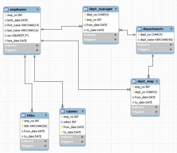
Concurrency & Locking
Introduction
Whether you're a DBA, DBDC or software developer you need to know how DB2 ensures data integrity. In this Assignment, we'll talk about one of the most important topics related to data integrity so locking mechanisms. Different types of SQL statements, commands and utilities require locks of a different type and size. There are basically two types of locking mechanisms in DB2, transaction locks, and claim/drain locks. We'll focus more on transaction locks since they're more important in software development and day-to-day work but you'll also learn some basics about claims and drains. In this and many upcoming Assignments, we'll use EMPLOYEE database created in "Loading a test database to DB2" Assignment. If you don't have it, be sure to upload it to your DB2 before starting this assignment.
Tasks
![]() 1. Create two SPUFI sessions with AUTOCOMMIT=NO:
- In the first one, retrieve employee records with IDs between 20000 and 20200 using different isolation levels (UR, CS, RS, and RR).
- After the query is done, leave the session open (don't issue COMMIT or ROLLBACK). This way you'll keep the lock on the data.
- In the second session try to issue SELECT and UPDATE statements on an employee with ID=20100.
- Each time use "DIS DB() SP() LOCKS/CLAIMERS" command to see lock details.
1. Create two SPUFI sessions with AUTOCOMMIT=NO:
- In the first one, retrieve employee records with IDs between 20000 and 20200 using different isolation levels (UR, CS, RS, and RR).
- After the query is done, leave the session open (don't issue COMMIT or ROLLBACK). This way you'll keep the lock on the data.
- In the second session try to issue SELECT and UPDATE statements on an employee with ID=20100.
- Each time use "DIS DB() SP() LOCKS/CLAIMERS" command to see lock details.
![]() 2. Create two SPUFI sessions with AUTOCOMMIT=NO:
- In the first session UPDATE employee with ID = 20100.
- Leave the session open (don't issue COMMIT or ROLLBACK).
- In the second session try to SELECT IDs between 20000 and 20200 using four isolation levels.
2. Create two SPUFI sessions with AUTOCOMMIT=NO:
- In the first session UPDATE employee with ID = 20100.
- Leave the session open (don't issue COMMIT or ROLLBACK).
- In the second session try to SELECT IDs between 20000 and 20200 using four isolation levels.
![]() 3. Create another EMPLOYEE table and populate it with data:
- Make user that one table has LOCKSIZE=PAGE and the other LOCKSIZE=ROW.
- Use two SPUFI sessions to concurrently update employee with ID 20001 and 20002 in the table with LOCKSIZE=PAGE.
- Next, use two SPUFI sessions to concurrently update employee with ID 20001 and 280000 in the table with LOCKSIZE=PAGE.
- Next, use two SPUFI sessions to concurrently update employee with ID 20001 and 20002 in the table with LOCKSIZE=ROW.
- Each time display LOCKS status.
3. Create another EMPLOYEE table and populate it with data:
- Make user that one table has LOCKSIZE=PAGE and the other LOCKSIZE=ROW.
- Use two SPUFI sessions to concurrently update employee with ID 20001 and 20002 in the table with LOCKSIZE=PAGE.
- Next, use two SPUFI sessions to concurrently update employee with ID 20001 and 280000 in the table with LOCKSIZE=PAGE.
- Next, use two SPUFI sessions to concurrently update employee with ID 20001 and 20002 in the table with LOCKSIZE=ROW.
- Each time display LOCKS status.
![]() 4. Test locks against claims using UNLOAD Utility:
- Block a single row using SELECT with RR isolation level and run UNLOAD on EMTBEMPL table.
- Repeat the test, this time block a row with use of UPDATE operation.
- Repeat the test again, this time run UNLOAD utility first and then quickly block employee with ID = 280000 with the UPDATE operation.
- Run unload utility again, then quickly block employee with ID = 12000 with the UPDATE operation.
4. Test locks against claims using UNLOAD Utility:
- Block a single row using SELECT with RR isolation level and run UNLOAD on EMTBEMPL table.
- Repeat the test, this time block a row with use of UPDATE operation.
- Repeat the test again, this time run UNLOAD utility first and then quickly block employee with ID = 280000 with the UPDATE operation.
- Run unload utility again, then quickly block employee with ID = 12000 with the UPDATE operation.
![]() 5. Using SPUFI sessions and DSNTEP2 batch job simulate a scenario in which transactions timeout due to RS and RR isolation level. In other words, test the behavior of RS and RR levels for UPDATE, INSERT, and DELETE statements.
- Don't forget to do an analysis of "DIS DB() SP() LOCKS" command.
5. Using SPUFI sessions and DSNTEP2 batch job simulate a scenario in which transactions timeout due to RS and RR isolation level. In other words, test the behavior of RS and RR levels for UPDATE, INSERT, and DELETE statements.
- Don't forget to do an analysis of "DIS DB() SP() LOCKS" command.
![]() 6. Answer following questions:
- Describe four concurrency problems: lost update, uncommitted read, non-repeatable read, phantom read.
- Describe four isolation levels: UR, CS, RS, and RR.
- What are the possible locks sizes?
- How locks on the row/page level influence locking on the partition/tablespace/table level?
- List possible claim classes that DB2 utilities use.
- List 5 factors that influence how DB2 locks the data.
- What's a lock escalation?
- What's a deadlock?
- What's a claim?
- What's a drain?
6. Answer following questions:
- Describe four concurrency problems: lost update, uncommitted read, non-repeatable read, phantom read.
- Describe four isolation levels: UR, CS, RS, and RR.
- What are the possible locks sizes?
- How locks on the row/page level influence locking on the partition/tablespace/table level?
- List possible claim classes that DB2 utilities use.
- List 5 factors that influence how DB2 locks the data.
- What's a lock escalation?
- What's a deadlock?
- What's a claim?
- What's a drain?
Hint 1-6
In SPUFI each user session can serve as a simulation of a single transaction. Therefore you can use the trick with multiple SPUFI sessions as a simulation of various concurrency scenarios. Make sure you set AUTOCOMMIT=NO and perform ROLLBACK each time. This way you'll be also able to test INSERT, DELETE, and UPDATE statements. When it comes to locking - be sure to check "Concurrency and locks" and "Claims and drains" chapters in "DB2 for z/OS: Managing Performance".
Solution 1
How SELECT blocks rows in regard to SELECT and UPDATE statement:
| Isolation level | SELECT | UPDATE | LOCKINFO | CLAIMINFO |
|---|---|---|---|---|
| UR | OK | OK | No lock | CS,C |
| CS | OK | OK | H-IS,P,C | CS,C |
| RS | OK | TIMEOUT | H-IS,P,C | CS,C |
| RR | OK | TIMEOUT | H-S,P,C | RR,C |
Using "/db2pref DIS DB(EMDBEMPL) SP(EMTSEMPL) LOCKS" and "/db2pref DIS DB(EMDBEMPL) SP(EMTSEMPL) CLAIMERS" you can display information lock and claim info for a particular request. As you can see using RS and RR in your read request will block any UPDATE operation on the row set you're fetching. Detailed description on what LOCKINFO and CLAIMINFO mean is available in the document describing DSNT361I message – you can search google for it.
Solution 2
How UPDATE blocks rows in regard to SELECT statement:
| Isolation level | SELECT |
|---|---|
| UR | OK |
| CS | TIMEOUT |
| RS | TIMEOUT |
| RR | TIMEOUT |
CLAIMINFO: (CS,C), (WR,C) LOCKINFO: H-IX,P,C If you'll display claiminfo with both session active and UR in SELECT statement you'll see that CLAIMINFO still shows CS although we'll simulated dirty read scenario. It's because CLAIMINFO doesn't show isolation level but "claim class". CS is a claim class for SELECTs issued with UR, CS, and RS, only RR has a different class in selects (RR). See "Claims and drains" chapter in "DB2 for z/OS: Managing Performance".
Solution 3
The results are not surprising: - Updating ID 20001 and 20002 in the table with LOCKSIZE=PAGE – Timeout. - Updating ID 20001 and 280000 in the table with LOCKSIZE=PAGE – Success. - Updating ID 20001 and 20002 in the table with LOCKSIZE=ROW – Success. If we investigate a little bit further we'll notice that the lock ends somewhere between IDs 20050 and 20100. So whenever you use LOCKSIZE=PAGE in your tables you must be aware that each lock blocks the entire page with usually consists of tens of records. Sometimes that's perfectly fine, after all, many tables are mainly read and rarely updated. But if a table is updated very often LOCKSIZE=ROW is the only acceptable option. In LOCKINFO we always have "H-IX,P,C". It's mentioned here to point out that the fact that we see "P (Partition)" lock here doesn't mean that the entire partition is locked for all operations, only some rows in it.
Solution 4
UNLOAD job:
//UTILLOAD EXEC DSNUPROC,SYSTEM=DB9G,UID='JSADEK.UNLOAD1' <-- DB2 SYS //STEPLIB DD DISP=SHR,DSN=DSN910.SDSNLOAD //SYSUT1 DD DISP=(,PASS),SPACE=(CYL,(20,80)) <-- SORT WRK DS //SORTWK01 DD DISP=(,PASS),SPACE=(CYL,(20,80)) <-- SORT WRK DS //SORTWK02 DD DISP=(,PASS),SPACE=(CYL,(20,80)) <-- SORT WRK DS //SORTWK03 DD DISP=(,PASS),SPACE=(CYL,(20,80)) <-- SORT WRK DS //SORTOUT DD DISP=(,PASS),SPACE=(CYL,(20,80)) <-- SORT WRK DS //SYSMAP DD DISP=(,PASS),SPACE=(CYL,(20,80)) <-- MAPPING WRK //SYSERR DD DISP=(,PASS),SPACE=(CYL,(20,80)) <-- ERROR WRK //RNPRIN01 DD SYSOUT=* <-- SORT MESSAGES //STPRIN01 DD SYSOUT=* <-- SORT MESSAGES //UTPRINT DD SYSOUT=* <-- SORT MESSAGES //SYSDISC DD SYSOUT=* <-- RECORDS NOT LOADED BY THE UTILITY //SYSPRINT DD SYSOUT=* <-- DB2 UTIL OUTPUT MESSAGES //SYSREC DD DSN=&&TEMP, // DISP=(,DELETE,DELETE), // SPACE=(CYL,(5,5),RLSE), // UNIT=SYSDA //SYSIN DD * <-- CONTROL STATEMENTS UNLOAD TABLESPACE EMDBEMPL.EMTSEMPL FROM TABLE "MPDB"."EMTBEMPL"
We don't care about the actual unload therefore we can use temporary data set in SYSREC. - Select with RR: OK - UPDATE block before UNLAOD: TIMEOUT - UPDATE block for a row that wasn't yet processed by UNLOAD: TIMEOUT - UPDATE block for a row that was already processed by UNLOAD: OK This task shows how a claim (UNLOAD utility) coexist and cooperates with a standard transaction lock (UPDATE and SELECT statements). Unload job doesn't interfere with any SELECT operations, it also allows updates, inserts, and deletes, but it will only read the commited data. So if some transaction locks a row for a long enough time, UNLOAD will abend due to timeout. UNLOAD utility by default uses UTRW claim which allows both read and update operations. This means that during UNLOAD rows can be added, removed or modified. If you desire to have an exact copy of a table from a given point in time you can use SHRLEVEL REFERENCE. Remember that each Utility locks the data in a different way. Also, claims may differ depending on the Utility options you've used and the object on which Utility works. Therefore, before running any Utility be sure to check how it handles concurrency in "DB2 for z/OS: Utility Guide and Reference".
Solution 5
The procedure for simulating timeouts for RS and RR can look as follows: - Tran1 - Using SPUFI session block employee record with ID=11000 using SELECT with RR isolation level. This way SELECTs in Transaction #2 will work while UPDATE no. - Tran2 - Run SQL via a batch job that: SELECTs IDs 499900-500100 with RR isolation level. Next, tries to update ID with 11000 and then reads IDs 499900-500100 again. - Tran3 - Run the second job with SQL that tries to update employee with ID=499900. - Tran4 - Run the third job with SQL that tries to insert a new row with ID=500000. - Tran5 - Run the fourth job with SQL that tries to delete an employee with ID=499900.
| Isolation level | INSERT | UPDATE | DELETE |
|---|---|---|---|
| UR in Tran2 | OK | OK | OK |
| CS in Tran2 | OK | OK | OK |
| RS in Tran2 | OK | TIMEOUT | TIMEOUT |
| RR in Tran2 | TIMEOUT | TIMEOUT | TIMEOUT |
RS are RR similar in the fact that both isolation levels lock the entire set of fetched rows for the time the transaction is active (CS locks only the row that's currently read). The difference lies in what operations are allowed between subsequent selects in the operation. This is a subtle difference but it makes a difference in COBOL programs so as a developer or DBA you must understand it. ________________________________________ Transaction #1 (SPUFI): SET SCHEMA = 'MPDB' ; -- SELECT * FROM EMTBEMPL WHERE EMP_NO = 11000 WITH RR ; ________________________________________ Transaction #2 (Batch): SET SCHEMA = 'MPDB' ; -- SELECT * FROM EMTBEMPL WHERE EMP_NO >= 499900 AND EMP_NO <= 500100 WITH RR ; -- UPDATE EMTBEMPL SET FIRST_NAME = 'XXXX' WHERE EMP_NO = 11000 ; -- SELECT * FROM EMTBEMPL WHERE EMP_NO >= 499900 AND EMP_NO <= 500100 ; -- ROLLBACK ; ________________________________________ Transaction #3 (Batch): SET SCHEMA = 'MPDB' ; -- UPDATE EMTBEMPL SET FIRST_NAME = 'JAN' WHERE EMP_NO = 499900 ; -- ROLLBACK ; ________________________________________ Transaction #4 (Batch): SET SCHEMA = 'MPDB' ; -- INSERT INTO EMTBEMPL VALUES (500002,'1964-06-02','JAN','SADEK2','M','1985-11-21') ; -- ROLLBACK ; ________________________________________ Transaction #5 (Batch): SET SCHEMA = 'MPDB' ; -- DELETE FROM EMTBEMPL WHERE EMP_NO = 499900 ; -- ROLLBACK ; ________________________________________ LOCKINFO for test with isolation level RR:
NAME TYPE PART STATUS CONNID CORRID LOCKINFO -------- ---- ----- ----------------- -------- ------------ --------- EMTSEMPL TS 0001 RW TSO JSADEK H-IS,P,C - AGENT TOKEN 770 EMTSEMPL TS 0001 RW BATCH JSADEKT2 H-SIX,P,C - AGENT TOKEN 805 EMTSEMPL TS 0001 RW BATCH JSADEKT5 W-IX,P,03 - AGENT TOKEN 808 EMTSEMPL TS 0001 RW BATCH JSADEKT4 W-IX,P,02 - AGENT TOKEN 807 EMTSEMPL TS 0001 RW BATCH JSADEKT3 W-IX,P,01 - AGENT TOKEN 806 EMTSEMPL TS RW
Notice the LOCKINFO details. Tran2 is marked as SIX which means that the transaction currently holds (H) Share access (S) but wants (I) exclusive access (X). The last parameter indicates a waiting queue. TSO user and Tran2 currently hold locks. The other transactions wait in a queue in the order marked by digits.
Solution 6
The previous five tasks presented to you various aspects of locking. You should have now the basic understanding of how DB2 locks the data. More importantly, you know how complex the subject is and how to analyze locks in real-world scenarios. Here we'll do a brief summary of what we've learned so far. ________________________________________ - Describe four concurrency problems: lost update, uncommitted read, non-repeatable read, phantom read. - Lost update – Happens when transaction A updates the data and before the changes are committed transaction B updates it again. In DB2 this problem is not possible. - Uncommitted read – Also known as a dirty read. Means reading the data that's not yet committed. - Non-repeatable read – Happens when the data read in the transaction is removed before the transaction ends, therefore various SQL statements won't see it. - Phantom read – Happens when the subsequent queries in the same transaction see a different data. ________________________________________ - Describe four isolation levels: UR, CS, RS, and RR. UR: - Lowest level – gives the highest degree of concurrency. - Can read even data locked in X and U modes. - Does not create any locks. - Cannot ensure data integrity since the read data can be always rolled back. - Can be used only on SELECTs. Lowest isolation level for update operations is CS. - Possible problems: uncommitted read, non-repeatable read, phantom read. - Not-possible problems: loss of update. CS: – The default isolation level. - In case of SELECT, the row is released after fetch is done or UOW ends (records that are already read can be updated/removed). - In case of UPDATE, INSERT and DELETE, the row is locked until UOW ends. - Possible problems: non-repeatable read, phantom read. - Not-possible problems: loss of update, uncommitted read. RS: - Locks all the rows that will be read/updated. - The lock is held until UOW ends. - Prevents any DELETE operation on the data used by the query. - Possible problems: phantom read. - Not-possible problems: loss of update, uncommitted read, non-repeatable read. RR: - Locks all the rows that will be read/updated. - The highest level of isolation, the lowest level of concurrency. - The lock is held until UOW ends. - Prevents any INSERT, UPDATE, and DELETE operation on the data used by the query. - Possible problems: none. - Not-possible problems: phantom read, loss of update, uncommitted read, non-repeatable read. ________________________________________ - What are the possible locks sizes? Table space, Table, Partition, Page, Row, LOB, XML ________________________________________ - How locks on the row/page level influence locking on the partition/tablespace/table level? There are two types of locks: - Row/page locks – SQL statements like SELECT or UPDATE work on this lock level. - Tablespace/table/partition locks – Utilities and some SQL statements like ALTER work on this level. Basically, when you lock the data with UPDATE you set one lock on row/page level which blocks other operations which need row/page lock on the data. You also create a second lock on partition/tablespace/table level which prevents any operation that requires a lock of this size, so for example, ALTER TABLE statement or REORG UTILITY. ________________________________________ - List possible claim classes that DB2 utilities use. In "DB2 for z/OS: Utility Guide and Reference" you can see how each utility locks the data. Be sure to check them before using any Utility. Here are possible claim classes: - None: Object not affected by this utility. - RI: Referential Integrity. - CR: Claim the read claim class. - CW: Claim the write claim class. - DA: Drain all claim classes, no concurrent SQL access. - DR: Drain the repeatable read class, no concurrent access for SQL repeatable readers. - DDR: Dedrain the read claim class, no concurrent access for SQL repeatable readers. - DW: Drain the write claim class, concurrent access for SQL readers. - UTUT: Utility restrictive state, exclusive control. - UTRO: Utility restrictive state, read-only access allowed. - UTRW - Utility restrictive state, read-write access allowed. - CHKP (NO): Concurrently running applications do not see CHECK-pending status after commit. - CHKP (YES): Concurrently running applications enter CHECK-pending after commit. ________________________________________ - List 5 factors that influence how DB2 locks the data. You can find those in "Concurrency and locks" chapter in "DB2 for z/OS: Managing Performance": - The type of processing being performed. - The value of LOCKSIZE for the target table. - The isolation level of the plan, package, or statement. - The method of access to data. - Whether the application uses the SKIP LOCKED DATA option. ________________________________________ - What's a lock escalation? Lock escalation is a performance improvement mechanism. When a transaction wants to lock large enough number of rows or pages, DB2 replaces all those locks with a lock for the entire tablespace of partition. UTS (which nowadays should be always used) use partitioning, therefore, the lock escalation in modern databases happens on a partition level. LOCKSIZE and LOCKMAX tablespace allocation parameters define how fast lock escalation occurs. ________________________________________ - What's a deadlock? Deadlock happens when a transaction A needs record or a set of records which are locked by transaction B and transaction B cannot progress because it needs data locked by the transaction A. That's the simplest scenario. Of course, deadlocks can happen with more than two transactions. Deadlocks are relatively rare and are an effect of a bad application design, therefore, there should be always fixed. ________________________________________ - What's a claim? DB2 claims/drains are similarly to transactions locks a mechanism of locking resource, just on a different level. The claim is an indicator that a particular resource is now in use. For example that some transaction or Utility uses a particular partition. Such claim defines what other operations are allowed on such a partition. ________________________________________ - What's a drain? Drains work similarly to drains. The main difference is that claims allow other claimers to access the object (if the claim is compatible) while drains prevent particular claim requests. Some utilities issue drains to ensure that nothing accesses the object while it's processed by the utility.
DB2 Performance - Basics
Introduction
One of the main DB2 strengths is its performance, thanks to its design, implementation of various performance improving techniques and of course, state of art mainframe I/O speed, DB2 is the fastest database on the market. Of course, that's only one part of the equation. Equally important, if not more, is the database and query design. In this Assignment, we'll go through the main rules regarding SQL queries performance. Some of them are crucial for the working of every database, some are little tweaks which may be not worth implementing in some cases. Still, for every COBOL developer or a DBA, this is a must-have knowledge. Performance in any area of any system is a highly subjective matter. Different z/OS or DB2 version may give different performance. Different hardware configuration and disk matrixes have different performance. And of course, the results will be hugely different if you're using zPDT instead of the real mainframe with its I/O and processor power. Therefore, remember that below values and % differences shouldn't be considered as universal, rather as a proof of the importance of each of the presented performance tweaks. Also, remember that query optimization is done when queries are implemented into an application program or script which will run regularly in the production environment. For "one-run" queries, optimization is most often not worth the time.
Tasks
![]() 1. Rule #1: Query only the data you absolutely need.
- JOIN EMTBEMPL & EMTBSLRY tables. Display 2000 employee records with "SELECT *".
- Then repeat the query but extract only FIRST_NAME, LAST_NAME, SALARY, FROM_DATE, and TO_DATE columns.
- Compare the performance of those two queries using the method of your own choice. The simplest method is described in Hint#1.
1. Rule #1: Query only the data you absolutely need.
- JOIN EMTBEMPL & EMTBSLRY tables. Display 2000 employee records with "SELECT *".
- Then repeat the query but extract only FIRST_NAME, LAST_NAME, SALARY, FROM_DATE, and TO_DATE columns.
- Compare the performance of those two queries using the method of your own choice. The simplest method is described in Hint#1.
![]() 2. Rule #2: Use EXPLAIN for query optimization.
- Create EXPLAIN tables under your ID.
- Select FIRST_NAME, LAST_NAME, and the SALARY of all employees who are working on "Assistant Engineer" position.
- How much processor time and service units this query is predicted to consume?
- How much did it really consumed?
- How many predicates were used and which category they are?
- How many SORTs were done?
- Accordingly to what columns records were sorted?
- How many indexes were used during the query?
2. Rule #2: Use EXPLAIN for query optimization.
- Create EXPLAIN tables under your ID.
- Select FIRST_NAME, LAST_NAME, and the SALARY of all employees who are working on "Assistant Engineer" position.
- How much processor time and service units this query is predicted to consume?
- How much did it really consumed?
- How many predicates were used and which category they are?
- How many SORTs were done?
- Accordingly to what columns records were sorted?
- How many indexes were used during the query?
![]() 3. Rule #3: Avoid tablespace scans.
- Repeat the same test as in Task#1. This time query only 100 employees.
- Use WHERE clause in the first test.
- In the second test, use FETCH FIRST clause to extract the same number of rows as in the first test.
- Use EXPLAIN statement to analyze both statements.
- What's the difference between those two queries?
3. Rule #3: Avoid tablespace scans.
- Repeat the same test as in Task#1. This time query only 100 employees.
- Use WHERE clause in the first test.
- In the second test, use FETCH FIRST clause to extract the same number of rows as in the first test.
- Use EXPLAIN statement to analyze both statements.
- What's the difference between those two queries?
![]() 4. Myth #1: Code predicates in order of restrictiveness.
- You want to find a record of a woman with the last name "Jonsson" that was born in 1962.
- Display all records that match these selection criteria using different selection order. For example, first test for the last name, then gender and then birth date and the other way around.
4. Myth #1: Code predicates in order of restrictiveness.
- You want to find a record of a woman with the last name "Jonsson" that was born in 1962.
- Display all records that match these selection criteria using different selection order. For example, first test for the last name, then gender and then birth date and the other way around.
![]() 5. Rule #4: JOIN order matters.
- Display all employees who are currently employed on "Senior Engineer" position and earn less than 50000 USD/year.
- Test different JOIN orders.
5. Rule #4: JOIN order matters.
- Display all employees who are currently employed on "Senior Engineer" position and earn less than 50000 USD/year.
- Test different JOIN orders.
![]() 6. Myth #2: If you need to issue multi-table queries, use JOINs.
- Display all employees who are currently earning 120000 USD/year and are working in the 'Development' department.
- Realize the query using WHERE clause and then using JOIN. Compare the results.
6. Myth #2: If you need to issue multi-table queries, use JOINs.
- Display all employees who are currently earning 120000 USD/year and are working in the 'Development' department.
- Realize the query using WHERE clause and then using JOIN. Compare the results.
![]() 7. Compare the performance of various multi-table query techniques.
- Display employees alongside with their salary history who have ever worked in the "Development" department and now earn 120000 USD/year or more. Test the query performance in following ways:
- Using WHERE keyword.
- Using JOINs.
- Using WITH keyword for subqueries.
- Using FROM keyword for subqueries - see Hint.
7. Compare the performance of various multi-table query techniques.
- Display employees alongside with their salary history who have ever worked in the "Development" department and now earn 120000 USD/year or more. Test the query performance in following ways:
- Using WHERE keyword.
- Using JOINs.
- Using WITH keyword for subqueries.
- Using FROM keyword for subqueries - see Hint.
![]() 8. Rule #5: Use correlated and uncorrelated queries appropriately.
- Select all employees on 'Senior Engineer' position which are still working in this role.
- Use correlated and uncorrelated query for this purpose and measure the difference.
8. Rule #5: Use correlated and uncorrelated queries appropriately.
- Select all employees on 'Senior Engineer' position which are still working in this role.
- Use correlated and uncorrelated query for this purpose and measure the difference.
![]() 9. Rule #6: Avoid sorting unless necessary.
- Display all employees who are currently working under 'Sanjoy Quadeer' manager.
- Repeat the query but this time display them in order of their birth dates.
9. Rule #6: Avoid sorting unless necessary.
- Display all employees who are currently working under 'Sanjoy Quadeer' manager.
- Repeat the query but this time display them in order of their birth dates.
![]() 10. Rule #7: Avoid functions and data conversion unless necessary.
- Modify the query from Task#9. Display employee name in upper-case. Also, add 10 years to the birth date and display it EUR format.
10. Rule #7: Avoid functions and data conversion unless necessary.
- Modify the query from Task#9. Display employee name in upper-case. Also, add 10 years to the birth date and display it EUR format.
![]() 11. Rule #8: Avoid unnecessary JOINs.
- Display FIRST_NAME and LAST_NAME of all employees who currently earn more than 100000 USD/year.
- Compare the performance of a query using JOIN and a subquery with IN clause.
11. Rule #8: Avoid unnecessary JOINs.
- Display FIRST_NAME and LAST_NAME of all employees who currently earn more than 100000 USD/year.
- Compare the performance of a query using JOIN and a subquery with IN clause.
Hint 1
There are various methods and tools for performance measurement. Most of them are payed, if you have a tool like that using it is probably the best choice. If not, don't worry, you can make a real test using SPUFI or DSNTEP2. All you need to do is to get system time just before and after the query using "SELECT CURRENT TIMESTAMP FROM SYSIBM.SYSDUMMY1;" This way you can calculate how much time each query used. It's of course not as accurate or detailed measurement as in professional tools but it enables you to clearly see a difference between test cases, and that's what really matters. An even easier way is to simply take a look at CPU usage of the DSNTEP2 job ("CPU" column in job output). The results here are less accurate but you'll still be able to compare the performance of test cases.
Hint 2
SQL needed for allocating tables used by EXPLAIN statement is available in DSNTESC sample member in SDSNSAMP library. All you need to do is to create a new database under you ID where you'll keep the tables and select the appropriate names for tablespaces and tables. The detailed description of all EXPLAIN tables is available in "Appendix B. DB2-supplied user tables" of "DB2 for z/OS: Managing Performance". Also, be sure to check "Investigating SQL performance by using EXPLAIN" chapter in the same document.
Hint 7
Similarly to WITH keyword you can use SELECTs instead of a table name in FROM clause, for example: SELECT E.FIRST_NAME, E.LAST_NAME, S.SALARY FROM EMTBEMPL E, ( SELECT EMP_NO, SALARY FROM EMTBSLRY WHERE SALARY >= 120000 ) S, WHERE S.EMP_NO = E.EMP_NO ;
Solution 1
Example DSNTEP2 job:
//JSADEKT2 JOB NOTIFY=&SYSUID //RUNSQL EXEC PGM=IKJEFT1B,REGION=0M //STEPLIB DD DISP=SHR,DSN=DSN910.DB9G.RUNLIB.LOAD // DD DISP=SHR,DSN=DSN910.SDSNLOAD //SYSTSPRT DD SYSOUT=* //SYSPRINT DD SYSOUT=* //SYSUDUMP DD SYSOUT=* //SYSTSIN DD * DSN SYSTEM(DB9G) RUN PROGRAM(DSNTEP2) PLAN(DSNTEP91) - PARMS('/ALIGN(LHS) MIXED') //SYSIN DD * SET SCHEMA = 'MPDB' ; -- SELECT CURRENT TIMESTAMP FROM SYSIBM.SYSDUMMY1 ; -- SELECT * FROM EMTBEMPL E JOIN EMTBSLRY S ON E.EMP_NO = S.EMP_NO WHERE E.EMP_NO >= 20000 AND E.EMP_NO < 22000 ; -- SELECT CURRENT TIMESTAMP FROM SYSIBM.SYSDUMMY1 ;
Test results: - SELECT * - 00.00.28.586545 - SELECT cols - 00.00.21.086120 As the above test proves, extracting selected columns speeds up the query by 25% in this case. Accordingly to the "Query only the data you absolutely need" rule, "SELECT *" is absolutely prohibited in applications or any scripts which run regularly in the production environment. In the case of single queries via SPUFI and such – don't worry about it, you can use "SELECT *" here. That's also important because using "SELECT *" will cause a serious error in case any column is added or removed from the table. Of course, this rule also says that you shouldn't fetch rows you don't need, not only columns.
Solution 2
SQL:
SET SCHEMA = 'MPDB' ; -- EXPLAIN ALL FOR SELECT E.FIRST_NAME, E.LAST_NAME, S.SALARY FROM EMTBEMPL E JOIN EMTBSLRY S ON S.EMP_NO = E.EMP_NO JOIN EMTBTITL T ON T.EMP_NO = E.EMP_NO WHERE T.TO_DATE = '9999-01-01' AND S.TO_DATE = '9999-01-01' AND T.TITLE = 'Assistant Engineer' ; -- SELECT * FROM JSADEK.DSN_STATEMNT_TABLE WHERE EXPLAIN_TIME > CURRENT TIMESTAMP - 1 MINUTE ; SELECT * FROM JSADEK.DSN_PREDICAT_TABLE WHERE EXPLAIN_TIME > CURRENT TIMESTAMP - 1 MINUTE ; SELECT * FROM JSADEK.DSN_FILTER_TABLE WHERE EXPLAIN_TIME > CURRENT TIMESTAMP - 1 MINUTE ; SELECT * FROM JSADEK.DSN_SORT_TABLE WHERE EXPLAIN_TIME > CURRENT TIMESTAMP - 1 MINUTE ; SELECT * FROM JSADEK.DSN_SORTKEY_TABLE WHERE EXPLAIN_TIME > CURRENT TIMESTAMP - 1 MINUTE ; SELECT * FROM JSADEK.PLAN_TABLE WHERE BIND_TIME > CURRENT TIMESTAMP - 1 MINUTE ; -- ROLLBACK ;
The above six EXPLAIN tables are probably the most useful for query optimization (there are 18 in total). If you don't want to save the results of EXPLAIN for good you can use SQL as shown above. ROLLBACK ensures that changes are not committed and WHERE clauses ensure that you exclude any other records which reside in the EXPLAIN tables. ________________________________________ - How much processor time and service units this query is predicted to consume? In DSN_STATEMNT_TABLE you can view an estimated cost of running a query. You can also see there how accurate the calculation are:
COST_CATEGORY PROCMS PROCSU REASON -+---------+---------+---------+---------+---------+------ B 66 344 TABLE CARDINALITY
Category B states that DB2 had to use default values for calculations and the estimate is not as accurate as if could be. The REASON states that it is so because of missing statistics. DB2 estimated that query will take 66ms or 344 CPU SU. ________________________________________ - How much did it really consumed? In comparison, the actual job: CPU = 0.9 min, SERV = 2848K That's a lot more than estimation but it's not a surprise. DB2 won't be able to calculate cost effectively without statistics. How it can know the cost of sorts of joins if it doesn't even know how many records are in each joined table? Of course, other processing is also going on in the job, even writing all those records to the output consumed a lot of CPU so some variations between results from EXPLAIN and the actual benchmark should be always expected. ________________________________________ - How many predicates were used and which category they are? DSN_FILTER_TABLE and DSN_PREDICAT_TABLE can help us here. We can see that query has 7 predicates in total. 6 of them (excluding AND) are available in DSN_FILTER_TABLE where we can see what stage they are:
PREDNO STAGE +---------+----- 2 STAGE1 4 STAGE1 5 MATCHING 3 STAGE1 6 STAGE1 7 STAGE2
Using PREDNO we can connect them to the predicates in DSN_PREDICAT_TABLE.
PREDNO TEXT ---+----------+---------+---------+ 1 (T.EMP_NO=S.EMP_NO AND ((((T 2 T.TO_DATE='9999-01-01' 3 S.TO_DATE='9999-01-01' 4 T.TITLE='Assistant Engineer' 5 T.EMP_NO=E.EMP_NO 6 S.EMP_NO=E.EMP_NO 7 T.EMP_NO=S.EMP_NO
So we have only one Stage 1 Indexable predicate (MATCHING), 4 stage 1 predicates and one stage 2 predicate. This is a strong indicators that the query can be optimized. At least on the first glance, in reality, even predicates marked STAGE1 here sometimes take advantage of an index. To be certain about that you check PLAN_TABLE where you can find what indexes were actually used in the query. ________________________________________ - How many SORTs were done? Two, both DSN_SORT_TABLE and DSN_SORTKEY_TABLE have four records but as you can see in SORTNO column there was actually only two sorts done. ________________________________________ - Accordingly to what columns records were sorted? In the DSN_SORTKEY_TABLE table, we can see that all sorts were done accordingly to EMP_NO column, one for EMTBSLRY table and one for EMTBTITL table. ________________________________________ - How many indexes were used during the query? PLAN_TABLE stores information about the query access path. We can find there what indexes were used during for the query. In this case, only one index was used, EMI1EMPL. ________________________________________ This Task only scratches the surface of the information available via EXPLAIN command and how they can be used. But the main thing is to know about the possibilities EXPLAIN provides and to use it on regular basis. This way, you'll become more and more familiar with it and you'll start seeing connections between values there and query performance that are invisible on the first sight.
Solution 3
SQL:
SET SCHEMA = 'MPDB' ; -- SELECT CURRENT TIMESTAMP FROM SYSIBM.SYSDUMMY1 ; -- SELECT E.FIRST_NAME, E.LAST_NAME, S.SALARY, S.FROM_DATE, S.TO_DATE FROM EMTBEMPL E JOIN EMTBSLRY S ON E.EMP_NO = S.EMP_NO -- WHERE E.EMP_NO >= 10001 AND E.EMP_NO <= 10100 ; FETCH FIRST 984 ROWS ONLY ; -- SELECT CURRENT TIMESTAMP FROM SYSIBM.SYSDUMMY1 ;
DSNTEP2 test: - WHERE clause - 00.00.01.307824 - FETCH FIRST clause - 00.09.29.568696 One of the most important rules in query optimization is related to complex queries. A complex query is a query which consists of two or more subqueries. In this example, two queries are done. One where you extract employees with selected Ids and the second when those records are joined with the ones from EMTBSLRY table. You see the huge difference between those two queries. It's because in the case of WHERE the first sub-query extracted only 100 employee records and then the second sub-query – which was done when joining tables only extracted rows with EMP_NO present in those 100 records from the first sub-query. In case of FETCH FIRST the entire tables were joined. So the result of the first sub-query was over 300 000 employee records instead of 100. This means that JOIN was done on those 300 000 and in the result, we had nearly 3 000 000 rows after the join. It's only at this point that DB2 extracted first 984 rows and discarded the remaining 3 mln. This is an extreme example of the lack of query optimization but it shows a few important points: - Using FETCH FIRST clause in complex queries is usually a bad idea. - It's useful to review EXPLAIN statement in search for possible areas of improvement and to see from how your code is understood by DB2 Optimizer. - Using EXPLAIN, in PLAN_TABLE you can see ACCESSTYPE=R & PREFETCH=S which means that a tablespace scan was done. This means that the query had read the entire tablespace (EMTSSLRY in this case) in order to get the result it needs. - MATCHCOLS=0 means that there is no filtering in a given subquery, so that entire columns need to be read, which in case of the non-indexed column also results in a tablespace scan. - Tablespace scans always mean bad performance and they're usually can be easily avoided.
Solution 4
SQL:
SELECT * FROM EMTBEMPL WHERE GENDER = 'F' AND BIRTH_DATE BETWEEN '1962-01-01' AND '1962-12-31' AND LAST_NAME = 'Jonsson' ;
GENDER, BIRTH_DATE, LAST_NAME order: 00.00.05.477650 BIRTH_DATE, LAST_NAME, GENDER order: 00.00.05.157586 LAST_NAME, BIRTH_DATE, GENDER order: 00.00.05.124937 The rule "Code predicates in order of restrictiveness" is actually a myth. It's because no matter how you code you query, DB2 Optimizer reorganizes it in the most optimal way (accordingly to its algorithms), therefore the order in which you code them doesn't matter. It's worth mentioning here about buffer pools. When you test query on a real environment, buffer pools also influence its performance. The first time you issue the query buffer pool won't make much difference, but for subsequent selects some data may be still in the buffer and may make the query faster. Therefore, when you're making performance tests, you should always do multiple of them and take an average or medium value from them. If you're making an actual report from your improvements you can use simple procedure: - Perform the test 5 times. - Discard the highest and the lowest time. - Calculate an average from the other three times. Test results in this and upcoming Assignments were calculated from two or three tests.
Solution 5
EMTBSLRY + EMTBEMPL + EMTBTITL:
SELECT E.FIRST_NAME, E.LAST_NAME, S.SALARY FROM EMTBSLRY S INNER JOIN EMTBEMPL E ON E.EMP_NO = S.EMP_NO INNER JOIN EMTBTITL T ON T.EMP_NO = S.EMP_NO WHERE S.TO_DATE = '9999-01-01' AND S.SALARY < 50000 AND T.TO_DATE = '9999-01-01' AND T.TITLE = 'Senior Engineer' ;
EMTBTITL + EMTBEMPL + EMTBSLRY:
SELECT E.FIRST_NAME, E.LAST_NAME, S.SALARY FROM EMTBTITL T INNER JOIN EMTBEMPL E ON E.EMP_NO = T.EMP_NO INNER JOIN EMTBSLRY S ON S.EMP_NO = T.EMP_NO WHERE S.TO_DATE = '9999-01-01' AND S.SALARY < 50000 AND T.TO_DATE = '9999-01-01' AND T.TITLE = 'Senior Engineer' ;
EMTBEMPL + EMTBTITL + EMTBSLRY:
SELECT E.FIRST_NAME, E.LAST_NAME, S.SALARY FROM EMTBEMPL E INNER JOIN EMTBTITL T ON T.EMP_NO = E.EMP_NO INNER JOIN EMTBSLRY S ON S.EMP_NO = E.EMP_NO WHERE S.TO_DATE = '9999-01-01' AND S.SALARY < 50000 AND T.TO_DATE = '9999-01-01' AND T.TITLE = 'Senior Engineer' ;
EMTBSLRY + EMTBTITL + EMTBEMPL:
SELECT E.FIRST_NAME, E.LAST_NAME, S.SALARY FROM EMTBSLRY S INNER JOIN EMTBTITL T ON T.EMP_NO = S.EMP_NO INNER JOIN EMTBEMPL E ON E.EMP_NO = S.EMP_NO WHERE S.TO_DATE = '9999-01-01' AND S.SALARY < 50000 AND T.TO_DATE = '9999-01-01' AND T.TITLE = 'Senior Engineer' ;
EMTBTITL + EMTBSLRY + EMTBEMPL:
SELECT E.FIRST_NAME, E.LAST_NAME, S.SALARY FROM EMTBTITL T INNER JOIN EMTBSLRY S ON S.EMP_NO = T.EMP_NO INNER JOIN EMTBEMPL E ON E.EMP_NO = T.EMP_NO WHERE S.TO_DATE = '9999-01-01' AND S.SALARY < 50000 AND T.TO_DATE = '9999-01-01' AND T.TITLE = 'Senior Engineer' ;
EMTBSLRY + EMTBEMPL + EMTBTITL: 00.02.02.989588 EMTBTITL + EMTBEMPL + EMTBSLRY: 00.02.03.154619 EMTBEMPL + EMTBTITL + EMTBSLRY: 00.01.14.535020 EMTBSLRY + EMTBTITL + EMTBEMPL: 00.01.13.877516 EMTBTITL + EMTBSLRY + EMTBEMPL: 00.02.02.105809 If we'll take a look at subqueries for each table we'll see that: - EMTBEMPL - 300024 rows (no subquery here). - EMTBTITL - 85939 - EMTBSLRY - 20305 So in theory the fastest solution is to first join EMTBSLRY(20305) with EMTBTITL(85939) since those two intermediate tables are the smallest. Then the result which will be only 3546 rows should be joined with EMTBEMPL. This way we would minimize the number of row comparisons. But that's theory, in reality DB2 optimizer tries to do that for us and depending on the way we code SQL, on table statistic and available indexes it may choose very different access paths. Conclusion: - Keep table statistic always up to date, even in test environments. - Experiment with SQL code, DB2 Optimizer does not always selects the most optimal path.
Solution 6
WHERE version:
SELECT E.FIRST_NAME, E.LAST_NAME, S.SALARY, DP.DEPT_NAME FROM EMTBEMPL E WHERE E.EMP_NO = S.EMP_NO AND E.EMP_NO = DE.EMP_NO AND DE.DEPT_NO = DP.DEPT_NO AND S.TO_DATE = '9999-01-01' AND S.SALARY >= 120000 AND DE.TO_DATE = '9999-01-01' AND DP.DEPT_NAME = 'Development' ;
JOIN version:
SELECT E.FIRST_NAME, E.LAST_NAME, S.SALARY, DP.DEPT_NAME FROM EMTBEMPL E INNER JOIN EMTBSLRY S ON E.EMP_NO = S.EMP_NO INNER JOIN EMTBDPEM DE ON E.EMP_NO = DE.EMP_NO INNER JOIN EMTBDPRT DP ON DE.DEPT_NO = DP.DEPT_NO WHERE S.TO_DATE = '9999-01-01' AND S.SALARY >= 120000 AND DE.TO_DATE = '9999-01-01' AND DP.DEPT_NAME = 'Development' ;
WHERE version: 00.02.43.394793 JOIN version: 00.02.43.430298 As we can see using JOINs instead of complex WHERE statement didn't give any increase in performance. So we can safely assume that's just an another myth. After all, DB2 Optimizer processes both statements and if their logic match performs exactly the same operations on the data.
Solution 7
Using a simple WHERE clause:
SELECT E.FIRST_NAME, E.LAST_NAME, DP.DEPT_NAME, S.SALARY, S.FROM_DATE, S.TO_DATE FROM EMTBEMPL E, EMTBSLRY S, EMTBDPRT DP, EMTBDPEM DE WHERE E.EMP_NO = S.EMP_NO AND S.SALARY >= 120000 AND E.EMP_NO = DE.EMP_NO AND DE.DEPT_NO = DP.DEPT_NO AND DP.DEPT_NAME = 'Development' ;
Using standard JOINs:
SELECT E.FIRST_NAME, E.LAST_NAME, DP.DEPT_NAME, S.SALARY, S.FROM_DATE, S.TO_DATE FROM EMTBEMPL E INNER JOIN EMTBSLRY S ON E.EMP_NO = S.EMP_NO INNER JOIN EMTBDPEM DE ON E.EMP_NO = DE.EMP_NO INNER JOIN EMTBDPRT DP ON DE.DEPT_NO = DP.DEPT_NO WHERE S.SALARY >= 120000 AND DP.DEPT_NAME = 'Development' ;
Using WITH keyword for sub-selects:
WITH TSALARY AS ( SELECT EMP_NO, SALARY, FROM_DATE, TO_DATE FROM EMTBSLRY WHERE SALARY >= 120000 ), TDPRT AS ( SELECT DEPT_NO, DEPT_NAME FROM EMTBDPRT WHERE DEPT_NAME = 'Development' ), TDPEM AS ( SELECT D.EMP_NO FROM EMTBDPEM D, TDPRT T WHERE T.DEPT_NO = D.DEPT_NO ) SELECT E.FIRST_NAME, E.LAST_NAME, DP.DEPT_NAME, S.SALARY, S.FROM_DATE, S.TO_DATE FROM EMTBEMPL E, TSALARY S, TDPRT DP, TDPEM DE WHERE E.EMP_NO = S.EMP_NO AND E.EMP_NO = DE.EMP_NO ;
Using FROM keyword for sub-selects:
SELECT E.FIRST_NAME, E.LAST_NAME, DE.DEPT_NAME, S.SALARY, S.FROM_DATE, S.TO_DATE FROM EMTBEMPL E, ( SELECT EMP_NO, SALARY, FROM_DATE, TO_DATE FROM EMTBSLRY WHERE SALARY >= 120000 ) S, ( SELECT DEPT_NO, DEPT_NAME FROM EMTBDPRT WHERE DEPT_NAME = 'Development' ) DP, ( SELECT D.EMP_NO, DP.DEPT_NAME FROM EMTBDPEM D, ( SELECT DEPT_NO, DEPT_NAME FROM EMTBDPRT WHERE DEPT_NAME = 'Development' ) DP WHERE D.DEPT_NO = DP.DEPT_NO ) DE WHERE E.EMP_NO = S.EMP_NO AND E.EMP_NO = DE.EMP_NO ;
If you think that's kind of messy code – you're right. This coding technique is rarely used since as you can see, we do here a similar thing as in WITH clause and WITH is much more readable. So let's sum it up: - Using a simple WHERE clause: 00.03.12.646771 - Using standard JOINs: 00.03.12.190038 - Using WITH keyword for sub-selects: 00.01.41.617510 - Using FROM keyword for sub-selects: 00.03.11.940071 Does it mean that joining tables with WITH keyword is faster? No, actually all methods give a very similar results. The reason why WITH had the highest performance is that tables were joined there in a different way. We can get the same result by doing following modification:
SELECT E.FIRST_NAME, E.LAST_NAME, DP.DEPT_NAME, S.SALARY, S.FROM_DATE, S.TO_DATE FROM EMTBEMPL E INNER JOIN EMTBSLRY S ON E.EMP_NO = S.EMP_NO INNER JOIN EMTBDPEM DE ON S.EMP_NO = DE.EMP_NO INNER JOIN EMTBDPRT DP ON DE.DEPT_NO = DP.DEPT_NO WHERE S.SALARY >= 120000 AND DP.DEPT_NAME = 'Development' ;
Here only one operand was replced and we got a big increase in performance: From: "INNER JOIN EMTBDPEM DE ON E.EMP_NO = DE.EMP_NO" - 00.03.14.745537 To: "INNER JOIN EMTBDPEM DE ON S.EMP_NO = DE.EMP_NO" - 00.01.45.735514 Conclusion: - Experiment with predicates, DB2 Optimizer won't replace a well-coded SQL. - Using COUNT(*) you can check how many rows will be joined in each sub-query and then use this information to check a few SQL variations that seems to be the most optimal. - WITH clause is easy to code and clearly shows how the data will be joined which may be useful during query optimization. - Pay special attention to non-indexed columns since they can slow down you query the most like SALARY column in this example. - Always use EXPLAIN and review the most important aspects of the query such as predicate stages, used indexes, the need for sorting and so on, this information will often point you to the possible query optimizations.
Solution 8
Correlated query:
SELECT E.FIRST_NAME, E.LAST_NAME FROM EMTBEMPL E WHERE E.EMP_NO = ( SELECT T.EMP_NO FROM EMTBTITL T WHERE T.EMP_NO = E.EMP_NO AND T.TITLE = 'Senior Engineer' AND T.TO_DATE = '9999-01-01' ) ;
Uncorrelated query using IN:
SELECT E.FIRST_NAME, E.LAST_NAME FROM EMTBEMPL E WHERE E.EMP_NO IN ( SELECT T.EMP_NO FROM EMTBTITL T WHERE T.TITLE = 'Senior Engineer' AND T.TO_DATE = '9999-01-01' ) ;
Uncorrelated query using WITH:
WITH TTAB AS ( SELECT EMP_NO FROM EMTBTITL WHERE TITLE = 'Senior Engineer' AND TO_DATE = '9999-01-01' ) SELECT E.FIRST_NAME, E.LAST_NAME FROM EMTBEMPL E, TTAB T WHERE E.EMP_NO = T.EMP_NO ;
Correlated query: 00.02.52.299499 Uncorrelated query using IN: 00.01.28.488125 Uncorrelated query using WITH: 00.01.21.289452 This is one of the "it depends" rules. Generally when processing a large qunatity of data uncorrelated query always wins. But when you're fetching only one or a few rows correlated query may be actually faster. Also, you should know that DB2 can sometimes "de-correlate" the query to improve the performance, but not in all cases.
Solution 9
SQL:
WITH TEMPL AS ( SELECT EMP_NO FROM EMTBEMPL WHERE FIRST_NAME = 'Sanjoy' AND LAST_NAME = 'Quadeer' ), TDEPT AS ( SELECT DEPT_NO FROM EMTBDPMG D, TEMPL E WHERE E.EMP_NO = D.EMP_NO ) SELECT E.FIRST_NAME, E.LAST_NAME, E.BIRTH_DATE FROM EMTBEMPL E, TDEPT D, EMTBDPEM M WHERE D.DEPT_NO = M.DEPT_NO AND M.EMP_NO = E.EMP_NO ORDER BY E.BIRTH_DATE ;
Without sorting: 00.00.32.828268 With sorting: 00.00.34.715887 The result set in this example had only 20117 rows, therefore sorting was done fairly quickly. The general rule states that you should avoid sorting unless necessary, especially in application programs, still: - Sorting usually (it depends on the SQL) is done on the result set, so if the query result has only tens or hundreds of rows, sorting them won't affect the performance much. - DB2 sorts are faster then sorting data separately via DFSORT or internal sorting in your programs, therefore if you need to sort data, it's better to sort it via SQL.
Solution 10
SQL:
WITH TEMPL AS ( SELECT EMP_NO FROM EMTBEMPL WHERE FIRST_NAME = 'Sanjoy' AND LAST_NAME = 'Quadeer' ), TDEPT AS ( SELECT DEPT_NO FROM EMTBDPMG D, TEMPL E WHERE E.EMP_NO = D.EMP_NO ) SELECT UPPER(FIRST_NAME), UPPER(LAST_NAME), CHAR(BIRTH_DATE + 10 YEARS,EUR) FROM EMTBEMPL E, TDEPT D, EMTBDPEM M WHERE D.DEPT_NO = M.DEPT_NO AND M.EMP_NO = E.EMP_NO ;
Without functions: 00.00.32.828268 With functions: 00.00.34.652459 As you can see the performance hit from using a few functions is also very small. Remember that processor is very fast. I/O to RAM memory is generally considered 100 000 times faster than I/O to DASD. Because of that, some performance rules like this one and the one before, usually won't speed up the query much, but they'll enable you to save some processor power. This is, of course, unimportant in one-time queries, but if such SQL is done every day for tens or thousands of times, then even the smallest improvement may significantly reduce cost of a particular application.
Solution 11
JOIN version:
SELECT E.FIRST_NAME, E.LAST_NAME FROM EMTBEMPL E INNER JOIN EMTBSLRY S ON S.EMP_NO = E.EMP_NO WHERE SALARY > 100000 AND TO_DATE = '9999-01-01' ;
IN version:
SELECT FIRST_NAME, LAST_NAME FROM EMTBEMPL WHERE EMP_NO IN ( SELECT EMP_NO FROM EMTBSLRY WHERE SALARY > 100000 AND TO_DATE = '9999-01-01' ) ;
JOIN version: 00.00.50.732496 IN version: 00.00.48.729936 This example shows a situation in which you need to join a table for logic reasons. You don't need the actual salaries of all those people, you just need the names. In such cases, doing JOINs is usually not an optimal solution. IN clause didn't bring huge improvement but every saving in processor power is good.
DB2 Performance - Indexes
Introduction
It's time to focus on the most important performance improving structure in DB2 so indexes. An index is an additional data set which consists of one or more sorted columns from the given table and the pointers to the actual rows. Thanks to the fact that data in indexes is always sorted DB2 can use much faster search algorithms. Indexes also speed up all operation that requires sorting so ORDER BY, GROUP BY, DISTINCT etc. Indexes are generally divided into unique and non-unique and to single-column and multi-columns ones. Unique indexes are allocated for columns in which only unique values are allowed, they're the fastest one. Non-unique indexes should be used for columns in which duplicated values can exist, they're not as fast but also speed up the search a lot in comparison to standard search. Multi-column indexes are structures which store more than one column. If a query uses both columns in the right way, index which stores both of them give the best performance. Still, multi-column indexes they're less universal (harder to utilize by DB2) and can even slow down some queries, so usually a single column indexes are a better choice.
Tasks
![]() 1. Get the count of employees which earn between 50000 and 100000 USD/year
- Use only the EMTBSLRY table in the query and do not check for TO_DATE.
- Allocate the Index for SALARY column and repeat the query.
- Modify the query so now you also display names of all employees that earn between 50000 and 52000 USD/year and repeat the experiment.
1. Get the count of employees which earn between 50000 and 100000 USD/year
- Use only the EMTBSLRY table in the query and do not check for TO_DATE.
- Allocate the Index for SALARY column and repeat the query.
- Modify the query so now you also display names of all employees that earn between 50000 and 52000 USD/year and repeat the experiment.
![]() 2. Test the performance of multi-columns index:
- In the first query display the COUNT of employees with FIRST_NAME starting from 'M'.
- In the second query display the COUNT of employees with FIRST_NAME starting from 'M' and LAST_NAME starting with 'Z'.
Repeat the queries four times:
- With no indexes.
- With an index for FIRST_NAME column.
- With two indexes, one for FIRST_NAME and one for LAST_NAME column.
- With multi-column index for FIRST_NAME and LAST_NAME columns.
2. Test the performance of multi-columns index:
- In the first query display the COUNT of employees with FIRST_NAME starting from 'M'.
- In the second query display the COUNT of employees with FIRST_NAME starting from 'M' and LAST_NAME starting with 'Z'.
Repeat the queries four times:
- With no indexes.
- With an index for FIRST_NAME column.
- With two indexes, one for FIRST_NAME and one for LAST_NAME column.
- With multi-column index for FIRST_NAME and LAST_NAME columns.
![]() 3. Test index performance in four operations. On all rows from EMTBSLRY table where earnings are equal to or above 10000 USD/year:
- Issue SELECT, UPDATE, and DELETE operations on all those rows.
- Next INSERT a few thousand new rows into the table.
- Remember to ROLLBACK your changes.
- Repeat the activity with and without an index for SALARY column.
3. Test index performance in four operations. On all rows from EMTBSLRY table where earnings are equal to or above 10000 USD/year:
- Issue SELECT, UPDATE, and DELETE operations on all those rows.
- Next INSERT a few thousand new rows into the table.
- Remember to ROLLBACK your changes.
- Repeat the activity with and without an index for SALARY column.
![]() 4. Test SORT operations with and without an index:
- Fetch all records of employees who earn 120000 USD/year or more.
- Use GROUP BY, ORDER BY ASC, ORDER BY DESC, and DISTINCT operations on SALARY column.
- Repeat the queries with and without an index.
4. Test SORT operations with and without an index:
- Fetch all records of employees who earn 120000 USD/year or more.
- Use GROUP BY, ORDER BY ASC, ORDER BY DESC, and DISTINCT operations on SALARY column.
- Repeat the queries with and without an index.
![]() 5. Test the column order in multi-column indexes.
- Issue two queries. In the first one display EMP_NO and SALARY using EMP_NO as a predicate. In the second do the same but use SALARY as a predicate.
- Test both queries in four situations: Only with default primary key index; Using multi-column index with EMP_NO, SALARY order; Using multi-column index with SALARY, EMP_NO order; Using separate indexes for both columns.
5. Test the column order in multi-column indexes.
- Issue two queries. In the first one display EMP_NO and SALARY using EMP_NO as a predicate. In the second do the same but use SALARY as a predicate.
- Test both queries in four situations: Only with default primary key index; Using multi-column index with EMP_NO, SALARY order; Using multi-column index with SALARY, EMP_NO order; Using separate indexes for both columns.
Hint 1-5
Be sure to check "Designing indexes for performance" chapter in "DB2 for z/OS: Managing Performance".
Solution 1
Allocating index:
CREATE INDEX EMI2SLRY ON EMTBSLRY (SALARY ASC) USING STOGROUP SYSDEFLT ERASE YES FREEPAGE 50 PCTFREE 10 ;
SQL for the first test:
SELECT COUNT(*) FROM EMTBSLRY WHERE SALARY BETWEEN 50000 AND 100000 ;
Performance with no index: 00.00.52.058815 Performance with index: 00.00.21.799705 SQL for the second test:
SELECT E.FIRST_NAME, E.LAST_NAME, S.SALARY FROM EMTBEMPL E, EMTBSLRY S WHERE S.SALARY BETWEEN 50000 AND 51000 AND S.EMP_NO = E.EMP_NO ;
Performance with no index: 00.01.53.407009 Performance with index: 00.01.53.389126 Test #1 shows how much you can gain using an Index. Test #2 shows an example of how an addition of an index doesn't bring any benefit since it's not used in the access path anyway. As usual, it depends on your query. SALARY column will be probably read by a lot of different programs and at the same time it will be rarely updated which makes this column a perfect candidate for an index.
Solution 2
SQL 1:
SELECT COUNT(*) FROM EMTBEMPL WHERE FIRST_NAME LIKE 'M%' ;
SQL 2:
SELECT COUNT(*) FROM EMTBEMPL WHERE FIRST_NAME LIKE 'M%' AND LAST_NAME LIKE 'Z%' ;
No Index: - Q1: 00.00.09.806764 - Q2: 00.00.10.278097 Index for FIRST_NAME: - Q1: 00.00.01.090925 - Q2: 00.00.10.195092 Allocating an index for FIRST_NAME column gave nearly 10x better performance in the first query. In the one where both first and last name are checked the LAST_NAME column is the bottleneck. Two indexes: - Q1: 00.00.01.112001 - Q2: 00.00.00.925428 This is an interesting result (Those queries were ran multiple times with the same results). With two indexes a query which checks two columns is faster than the query which checks only one column, at least in this test. More importantly, we've proved that a query like that needs indexes for all predicates to perform really well. Multi-column index: - Q1: 00.00.01.281003 - Q2: 00.00.01.570325 This experiment proved that using multi-column index is not always a better choice than a single column one: - When it comes to performance it sometimes positively and sometimes negatively influences the performance. - It lowers performance in queries which test data from only one column. For example, if you'll test only FIRST_NAME multi-column index will always perform worse than standard index. - Therefore, you should be aware that when using multi-columns index to improve one query you may also decrease performance of other queries which would do better with two separate indexes. To sum it up, if you're creating a multi-column index for a specific, very important query which performs better with it, use it. For all the other cases standard indexes are probably a better choice.
Solution 3
SELECT:
SELECT COUNT(*) FROM EMTBSLRY WHERE SALARY >= 100000 ;
- Without index: 00.00.31.521562 - With index: 00.00.01.502076 UPDATE:
UPDATE EMTBSLRY SET SALARY = 0 WHERE SALARY >= 100000 ;
- Without index: 00.00.53.651367 - With index: 00.03.13.510613 DELETE:
DELETE FROM EMTBSLRY WHERE SALARY >= 100000 ;
- Without index: 00.01.40.958056 - With index: 00.03.08.099369 INSERT:
INSERT INTO EMTBSLRY SELECT EMP_NO, 500000, FROM_DATE + 50 YEAR, '9999-01-01' FROM EMTBSLRY WHERE SALARY >= 100000 ;
Primary key of EMTBSLRY table is made up of two columns EMP_NO and FROM_DATE, therefore there cannot be a duplicated records with the same values in both those columns and EMP_ID must exist in EMTBEMPL table. To overcome that restriction and INSERT a lot of test data you must modify FROM_DATE in a way so each Primary Key is unique. - Without index: 00.02.48.620695 - With index: 00.03.45.197064 You can see here "the dark side" of Indexes. Of course, each index needs an additional storage, but nowadays, that's not much of a cost. What's really important to remember is that index will always slow down INSERT, UPDATE, and DELETE operations. After all, now each operation needs to modify the data in two places. Without an index the UPDATE operation had to modify over 94000 rows, with index twice that much rows need to be updated. Especially costly are UPDATE and INSERT operations on indexes since in those case other records in the index must be also reorganized, which means an additional I/O even if you have a lot of free space left in your index. Therefore, before allocating an index you should carefully consider how a particular table is used. If a big percentage of operations there are updates than their cost may be significantly higher than a benefit of faster SELECT and FETCH operations.
Solution 4
GROUP BY:
SELECT COUNT(*), SALARY FROM EMTBSLRY WHERE SALARY >= 120000 GROUP BY SALARY ;
Without index: 00.00.33.739928 With index: 00.00.04.754668 ORDER BY ASC:
SELECT SALARY FROM EMTBSLRY WHERE SALARY >= 120000 ORDER BY SALARY ASC ;
Without index: 00.00.34.967743 With index: 00.00.05.588273 ORDER BY DESC:
SELECT SALARY FROM EMTBSLRY WHERE SALARY >= 120000 ORDER BY SALARY DESC ;
Without index: 00.00.33.315624 With index: 00.00.05.449460 DISTINCT:
SELECT DISTINCT(SALARY) FROM EMTBSLRY WHERE SALARY >= 120000 ;
Without index: 00.00.32.584947 With index: 00.00.04.775949 DB2 may perform sorting when you use JOIN, ORDER BY, GROUP BY, DISTINCT and UNION statements (UNION ALL doesn't performs sorting so if you can use it instead of UNION – do that). Index by definition is simply a sorted copy of a column therefore it can eliminate need for sort operations. When it comes to sorting recommendation it goes as follows: - The best option is to avoid sorting alltogether. - If you must do sorting, do it via SQL. - Never do sorting in your programs that SQL can do. It's also worth mentioning here about ASC and DESC keywords. Generally DB2 can do "Backward index scan" so it can utilize ASC index even when you sort in descending order, but as usual, it depends on the particular query if this will be actually done. Also a slight modification in the query (adding EMP_NO column) will prevent DB2 for using the our new index, at least in this case:
SELECT EMP_NO, SALARY FROM EMTBSLRY WHERE SALARY >= 120000 ORDER BY SALARY ASC ;
Without index: 00.00.34.956119 With index: 00.00.35.558678 Another worth mentioning aspect of idexes is index-only access. In case like the ones above when only columns from an index are read, DB2 won't even access the actual EMTBSLRY table, all the data will be read from the index.
Solution 5
Creating a multicolumn index for the third test:
CREATE INDEX EMI2SLRY ON EMTBSLRY (SALARY ASC, EMP_NO ASC) USING STOGROUP EMDBSTOG ERASE YES FREEPAGE 50 PCTFREE 10 ;
Query 1:
SELECT EMP_NO, SALARY FROM EMTBSLRY WHERE SALARY BETWEEN 100000 AND 200000 ;
Query 2:
SELECT EMP_NO, SALARY FROM EMTBSLRY WHERE EMP_NO BETWEEN 10000 AND 20000 ;
A Primary key index for EMP_NO: Q1: 00.01.34.270276 Q2: 00.01.40.166525 Multi-column index for EMP_NO & SALARY: Q1: 00.01.48.636213 Q2: 00.01.07.086389 Multi-column index for SALARY & EMP_NO: Q1: 00.01.06.796497 Q2: 00.01.56.015481 Two separate indexes: Q1: 00.01.35.681141 Q2: 00.01.40.386848 This Task shows how using multi-column indexes always speed up some queries and slow down the others, therefore using them is a risky business. It may turned out that by creating one index you get a huge performance increase in the query you're optimizing but at the same time you decrease performance of another much more important query. On the other hand, allocating two single column indexes can be nearly as fast as a multi-column one in some cases and doesn't create a risk of degraded performance in other queries. But as seen in this example, they're not always utilized in queries where a multi-column index would be. You can also see here how column order in a multi-column index affects different types of queries.
DB2 Performance - Predicates
Introduction
Predicates are simply an logical operators that define which data should be fetched from a database. Standard operators like '=', '>=', 'NOT' are predicates and also SQL specific keywords like DISTINCT, LIKE, or BETWEEN are also predicates. Predicates have a huge influence on query performance. They define at which stage of SQL processing data is excluded, what data is excluded, and how tables are joined with each other. Of course, the less data is processed the less I/O both to DASDs and RAM and the less I/O the better query performance.
Tasks
![]() 1. Answer following questions:
- List types of predicates in terms of range.
- Describe two stages of SQL processing.
- Find if following predicates are indexable and in which stages they're resolved: 'col < value', 'col1 IN col2', 'col LIKE 'text%', 'col LIKE '%text', 'col <> value', 'col BETWEEN value1 & value2', 'value BETWEEN col1 and col2'.
1. Answer following questions:
- List types of predicates in terms of range.
- Describe two stages of SQL processing.
- Find if following predicates are indexable and in which stages they're resolved: 'col < value', 'col1 IN col2', 'col LIKE 'text%', 'col LIKE '%text', 'col <> value', 'col BETWEEN value1 & value2', 'value BETWEEN col1 and col2'.
![]() 2. Display an average salary for employees which earn 120000 USD/year or more. Create three queries for this purpose, each using different predicate category:
- Stage 2 predicate.
- Stage 1 predicate.
- Stage 1 indexable predicate (You'll need to create an index).
- Compare the performance of those queries.
2. Display an average salary for employees which earn 120000 USD/year or more. Create three queries for this purpose, each using different predicate category:
- Stage 2 predicate.
- Stage 1 predicate.
- Stage 1 indexable predicate (You'll need to create an index).
- Compare the performance of those queries.
![]() 3. Check using COUNT function if there are any records in EMTBEMPL table where gender doesn't match either 'M' or 'F' value.
- Use Stage 1 and Stage 1 Indexable predicate for comparison.
3. Check using COUNT function if there are any records in EMTBEMPL table where gender doesn't match either 'M' or 'F' value.
- Use Stage 1 and Stage 1 Indexable predicate for comparison.
![]() 4. Display all employees hired in 1990 using different types of predicates. Compare their performance.
4. Display all employees hired in 1990 using different types of predicates. Compare their performance.
![]() 5. Optimize a sample query.
- Assume the following query will run regularly in the production environment. Your goal is to make it as fast as possible using the knowledge you've gained so far.
- Test performance gains after each optimization.
5. Optimize a sample query.
- Assume the following query will run regularly in the production environment. Your goal is to make it as fast as possible using the knowledge you've gained so far.
- Test performance gains after each optimization.
SELECT E.FIRST_NAME, E.LAST_NAME, S.SALARY FROM EMTBEMPL E, EMTBSLRY S, EMTBDPRT DP, EMTBDPEM DE WHERE E.EMP_NO = S.EMP_NO AND E.EMP_NO = DE.EMP_NO AND DE.DEPT_NO = DP.DEPT_NO AND S.SALARY >= 120000 AND DP.DEPT_NAME = 'Development' ;
Hint 1-4
Stages and various predicate classifications are presented in "Using predicates efficiently" chapter in "DB2 for z/OS: Managing Performance". Also, remember about the EXPLAIN statement through which you can check what predicates are used, what stage they are, what indexes are used and so on.
Solution 1
- List types of predicates in terms of range. Subquery predicates - Any predicate which includes a SELECT subquery. Equal predicates - '=', 'IS NULL', 'IS NOT DISTINCT'. Range predicates - '>', '>=', '<', '<=', 'LIKE', 'BETWEEN'. IN predicate - 'IN'. NOT predicate - Any predicate which includes NOT keyword. ________________________________________ - Describe two stages of SQL processing. The most important aspect of query optimization is using predicates and other SQL constructs in such a way to minimize the number of times data must be processed and to minimize the amount of data processed at each processing phase. When you issue a query the data is first read from an LDS VSAM data set (tablespace, indexspace or both) to Buffer Pool via Buffer Manager. At this point, the way you coded predicates doesn't matter. Next, it's moved from Buffer Pool to Data Manager. During this movement, some rows may be excluded (not moved to Data Manager). Obviously, the less data is moved at this point the less rows will have to be processed later at Stage 2 which has a big effect on query performance. Next, it's moved from the Data Manager to Relational Data Services where some higher level SQL processing is done, such as JOINs. Movement from Data Manager to Relational Data Services is Stage 2. Basically, the way you code predicates, their type and operands, define at what time of data processing the data excluded by the operands is really discarded from further processing. The sooner it happens the less data needs to be processed later. Predicates also define if the index will be used or not. Therefore we divide predicates on three types: - Indexable Stage 1 predicates. - Non-Indexable Stage 1 predicates. - Stage 2 predicates (stage 2 is always non-indexable). ________________________________________ - Find if following predicates are indexable and in which stages they're resolved: 'col < value', 'col1 IN col2', 'col LIKE value', '<>', 'col BETWEEN value1 & value2', 'value BETWEEN col1 and col2'. 'col < value' – Stage 1 Indexable 'col1 IN col2' – Stage 1 Indexable 'col LIKE 'text%' - Stage 1 Indexable 'col LIKE '%text' – Stage 1 'col <> value' - Stage 1 'col BETWEEN value1 AND value2' - Stage 1 Indexable 'value BETWEEN col1 AND col2' – Stage 2
Solution 2
The detailed list of predicates divided into three performance categories is avaialable in "Summary of predicate processing" chapter in "DB2 for z/OS: Managing Performance". Stage 2 'expression op value' predicate:
SELECT AVG(SALARY) FROM EMTBSLRY WHERE SALARY / 12 >= 10000 ;
Stage 1 'COL op noncol expr' predicate:
SELECT AVG(SALARY) FROM EMTBSLRY WHERE SALARY >= 240000 / 2 ;
Stage 2: 00.04.33.709005 Stage 1: 00.00.30.693163 Stage 1 Indexable: 00.00.00.205110 Of course there is an additional workload related to number calculations since in the first case expression must be resolved for each row, in the seconds DB2 can resolve it only once. But remember about the previous exercises, functions and calculation doesn't have nearly as big influence on performance as DASD I/O has. A good proff for that is that even adding a subquery won't slow down the main query as much as Stage 2 predicate:
SELECT AVG(SALARY) FROM EMTBSLRY WHERE SALARY >= ( SELECT 240000 FROM SYSIBM.SYSDUMMY1 ) / 2 ;
Result (Stage 1): 00.04.09.462814
Solution 3
Stage 1 predicate:
SELECT COUNT(*) FROM EMTBEMPL WHERE GENDER NOT IN ('F', 'M') ;
Stage 1 indexable predicate:
SELECT COUNT(*) FROM EMTBEMPL WHERE GENDER IN ('A','B','C','D','E','G','H','I','J','K', 'L','N','O','P','Q','R','S','T','U','V','W','X','Y','Z', ' ','a','b','c','d','e','g','h','i','j','k', 'l','n','o','p','q','r','s','t','u','v','w','x','y','z');
Stage 1: 00.00.04.528375 Stage 1 indexable: 00.00.00.103730 This is both stupid and a great example of how to code predicates. Stupid because no one spells entire alphabet to test for two letters. And great because if such query should run regularly on a system, hundreds of thousands of times each day, this is exactly what you should do. Of course, the second query doesn't contain all the options the first do. For example, it doesn't test for numbers. That just laziness, adding another 50 characters to it won't change the point made here.
Solution 4
Here are a few versions how can you realize the requested query:
SELECT FIRST_NAME, LAST_NAME FROM EMTBEMPL WHERE HIRE_DATE >= '1990-01-01' AND HIRE_DATE < '1991-01-01' ; ________________________________________ SELECT FIRST_NAME, LAST_NAME FROM EMTBEMPL WHERE HIRE_DATE BETWEEN '1990-01-01' AND '1990-12-31' ; ________________________________________ SELECT FIRST_NAME, LAST_NAME FROM EMTBEMPL WHERE CHAR(HIRE_DATE,ISO) LIKE '1990%' ; ________________________________________ SELECT FIRST_NAME, LAST_NAME FROM EMTBEMPL WHERE YEAR(HIRE_DATE) = 1990 ;
>= & < version: 00.00.19.917531 BETWEEN version: 00.00.19.611249 CHAR + LIKE version: 00.00.45.837969 YEAR version: 00.00.46.102615 From the above queries the first two versions use Stage 1 predicates and therefore are significantly faster. The last two queries may seem like Stage 1 since they're using '=' and LIKE but on the left side we don't have a column but a function so it's not 'col = value' but 'expression = value' which is Stage 2 predicate. Generally when it's recommended to use BETWEEN keyword for checking DATE, TIME, and TIMESTAMP data types since it's Stage 1 Indexable predicate and is slightly faster than using standard operators such as '<'.
Solution 5
Original SQL:
SELECT E.FIRST_NAME, E.LAST_NAME, S.SALARY FROM EMTBEMPL E, EMTBSLRY S, EMTBDPRT DP, EMTBDPEM DE WHERE E.EMP_NO = S.EMP_NO AND E.EMP_NO = DE.EMP_NO AND DE.DEPT_NO = DP.DEPT_NO AND S.SALARY >= 120000 AND DP.DEPT_NAME = 'Development' ;
Removing an unnecessary subquery:
SELECT E.FIRST_NAME, E.LAST_NAME, S.SALARY FROM EMTBEMPL E, EMTBSLRY S, EMTBDPEM D WHERE E.EMP_NO = S.EMP_NO AND E.EMP_NO = D.EMP_NO AND S.SALARY >= 120000 AND D.DEPT_NO = 'd005' ;
The first optimization is to remove one JOIN which is simply unnecessary. Department ID can be checked once with a single query so checking it each time doesn't have much sense. Also, department name is much more likely to change than department ID so we additionally avoid need for frequent query updates. The gain here is mainly caused due to EMTBSLRY table for which DB2 used tablespace scan earlier. Using JOINs instead of a complex WHERE:
SELECT E.FIRST_NAME, E.LAST_NAME, S.SALARY FROM EMTBEMPL E INNER JOIN EMTBSLRY S ON E.EMP_NO = S.EMP_NO INNER JOIN EMTBDPEM D ON E.EMP_NO = D.EMP_NO WHERE S.SALARY >= 120000 AND D.DEPT_NO = 'd005' ;
The next optimization we've checked is replacing AND with JOINs, just out of curiosity since it was proven a myth before. In this particular case, gains are also marginal so its safe to assume that it confirms that JOINs are faster than WHERE is a myth. Adding an index for SALARY column:
WITH TSLRY AS ( SELECT EMP_NO, SALARY FROM EMTBSLRY WHERE SALARY >= 120000 ORDER BY SALARY ) SELECT E.FIRST_NAME, E.LAST_NAME, S.SALARY FROM EMTBEMPL E INNER JOIN TSLRY S ON E.EMP_NO = S.EMP_NO INNER JOIN EMTBDPEM D ON E.EMP_NO = D.EMP_NO WHERE D.DEPT_NO = 'd005' ;
In case of table EMTBSLRY, we can safely allocate an index. It stores employee data which is very rarely updated so the additional cost of INSERT/UPDATE operation won't be high. Of course, allocating index is only part of the job. You must also redesign your query in a way so it uses the index. JOINs can influence how an index is used and even if a predicate fits "Stage 1 Indexable" category, it may not use the index if it's a multi-table query. In this example it wasn't enough to outsource EMTBSLRY subquery to WITH clause, we also had to use ORDER BY clause. Otherwise, the data would be received accordingly to EMP_NO index which is not an efficient choice here. Changing JOIN order & predicate reorganization:
WITH TSLRY AS ( SELECT EMP_NO, SALARY FROM EMTBSLRY WHERE SALARY >= 120000 ORDER BY SALARY ) SELECT E.FIRST_NAME, E.LAST_NAME, S.SALARY FROM TSLRY S INNER JOIN EMTBEMPL E ON S.EMP_NO = E.EMP_NO INNER JOIN EMTBDPEM D ON S.EMP_NO = D.EMP_NO WHERE D.DEPT_NO = 'd005' ;
Replacing single-column with multi-column index: At this point, further improvement seems ineffective, so it's time for the EXPLAIN. As shown below, there is still some room for improvement. It seems that the new index for SALARY table improves performance but still isn't the best choice. Let's replace it multi-column index for EMP_NO and SALARY columns since those are the ones we use in our query.
SELECT P.PREDNO, P.TEXT, F.STAGE, P.TYPE, P.JOIN, P.KEYFIELD FROM JSADEK.DSN_PREDICAT_TABLE P LEFT JOIN JSADEK.DSN_FILTER_TABLE F ON P.PREDNO = F.PREDNO WHERE P.EXPLAIN_TIME > CURRENT TIMESTAMP - 1 MINUTE AND F.EXPLAIN_TIME > CURRENT TIMESTAMP - 1 MINUTE ; -------+---------+---------+---------+---------+---------+---------+---------+- PREDNO TEXT STAGE TYPE -------+---------+---------+---------+---------+---------+---------+---------+- 2 D.DEPT_NO='D005' MATCHING EQUAL 3 S.EMP_NO=D.EMP_NO STAGE2 EQUAL 4 S.EMP_NO=E.EMP_NO STAGE2 EQUAL 4 S.EMP_NO=E.EMP_NO MATCHING EQUAL 5 MPDB.EMTBSLRY.SALARY>=120000 STAGE1 RANGE 6 D.EMP_NO=E.EMP_NO MATCHING EQUAL
This is also an example of how DB2 takes advantage of an index and still shows STAGE1 in the output of EXPLAIN statement. In PLAN_TABLE you can always see which indexes are really utilized. A new index:
CREATE INDEX EMI3SLRY ON EMTBSLRY (SALARY ASC, EMP_NO ASC) USING STOGROUP SYSDEFLT ERASE YES FREEPAGE 50 PCTFREE 10 ;
And the query, notice that now ORDER BY EMP_NO is used to correctly utilize the index:
WITH TSLRY AS ( SELECT EMP_NO, SALARY FROM EMTBSLRY WHERE SALARY >= 120000 ORDER BY EMP_NO ) SELECT E.FIRST_NAME, E.LAST_NAME, S.SALARY FROM TSLRY S INNER JOIN EMTBEMPL E ON S.EMP_NO = E.EMP_NO INNER JOIN EMTBDPEM D ON S.EMP_NO = D.EMP_NO WHERE D.DEPT_NO = 'd005' ;
You can have as many indexes as you wish for each table and DB2 will always select the one that seems the best choice for a particular query. In this case, a multi-column index performs the best, in other queries, the index for the SALARY column we've created previously would be better. But remember that each new index slows down update operations on the table. At the beginning we had a table and an index so only 2 I/Os were needed to update one record, now we have three indexes so 4 I/Os will be needed. So you must always weight the costs and benefits of using indexes, especially multi-column ones. Original SQL: 00.03.10.931448 Removing an unnecessary subquery: 00.01.29.261248 Using JOINs instead of a complex WHERE: 00.01.28.193672 Switching predicate positions in various ways: No gains Adding an index for SALARY column: 00.00.45.496306 Changing JOIN order & predicate reorganization: 00.00.34.188172 Replacing single-column with multi-column index: 00.00.07.114485 We've started with what seems to be a perfectly fine query which gets all employees from 'Development' department that has ever earned 120000 USD/year or more. By using few more and few less obvious optimization tricks we've been able to speed up the query from 3:11 to 0:07, which is 27 times faster! This Task presents how query optimization can look like. EXPLAIN statement is often referred to as the basis of query optimization. In reality, EXPLAIN can only give you some ideas on what you can/should do with the particular query. In the end, it all comes to understanding how DB2 processes queries and experimenting with various optimization tricks like we did here. Another reason why experimentation is necessary is that depending on the data, particular SQL code and DB2 statistics different optimization techniques will work. A technique which gives big performance gains in one case may decrease performance in others, therefore "each case is different" approach should be always used. When it comes to EXPLAIN the most time-effective method is to first play with various query variation using your experience and intuition benchmarking each version. Only when you are stuck and further modifications don't bring performance improvements, use EXPLAIN to analyze the most optimal version and see if there is something more that can be improved.